Adversarial Validation for Dataset Drift

Hello! Welcome to the seventh lesson in our module on "Advanced Feature Engineering Principles."

Introduction

In our last lesson, we put on our architect hats and learned how to design a feature engineering strategy from the ground up, balancing trade-offs between complexity, interpretability, and cost. We established a blueprint for creating features based on historical data.

However, a model's journey doesn't end in the research notebook. When deployed to production, it faces a constantly changing world. Data distributions that were stable during training can shift due to seasonality, changes in user behavior, or modifications in upstream data sources. This phenomenon is broadly known as distribution drift, and it's a primary reason why models degrade over time.

This lesson directly addresses the learning outcome: Apply adversarial validation to diagnose and quantify distribution drift between training, validation, and production datasets. We will learn a powerful and elegant technique that reframes the problem of detecting drift into a standard classification task, giving you a robust tool to ensure your models are built on a solid foundation and remain performant in the wild.

The Challenge of Distribution Drift

Imagine you train a model on data from January to May and plan to test it on data from June. If a major marketing campaign launched in late May changed the type of users signing up, your June data might have a different statistical profile than your training data. Your model, trained on the old "rules," may not generalize well. This is distribution drift.

From a more formal perspective, given a dataset of features $\mathbf{x}$ and labels $y$, the joint probability distribution is $P(\mathbf{x},y)$. Drift can occur in several ways. While the terminology can vary, it's useful to distinguish between a few key types:

• Covariate Shift: The distribution of the input features $P(\mathbf{x})$ changes, but the relationship between features and the target $P(y|\mathbf{x})$ remains the same. This is the most common type of drift and the one adversarial validation is especially good at detecting. (e.g., the average age of your user base changes).
• Prior Probability Shift: The distribution of the target variable $P(y)$ changes. (e.g., the baseline fraud rate in your system suddenly doubles).
• Concept Shift: The fundamental relationship between features and the target $P(y|\mathbf{x})$ changes. (e.g., a feature that was once a strong predictor of churn becomes irrelevant).

Adversarial validation provides a direct and intuitive way to test for these differences, particularly covariate shift.

The Adversarial Validation Framework

The core idea behind adversarial validation is simple yet brilliant. Instead of using complex statistical tests to compare distributions, we rephrase the question: "Can a machine learning model tell the difference between my training data and my production data?"

If a classifier can easily distinguish between samples from the two datasets, it implies there are systematic differences in their feature distributions. If the classifier can't do any better than random guessing, the datasets are likely indistinguishable and come from a similar distribution.

To build our foundational understanding, let's watch a video that explains this process.

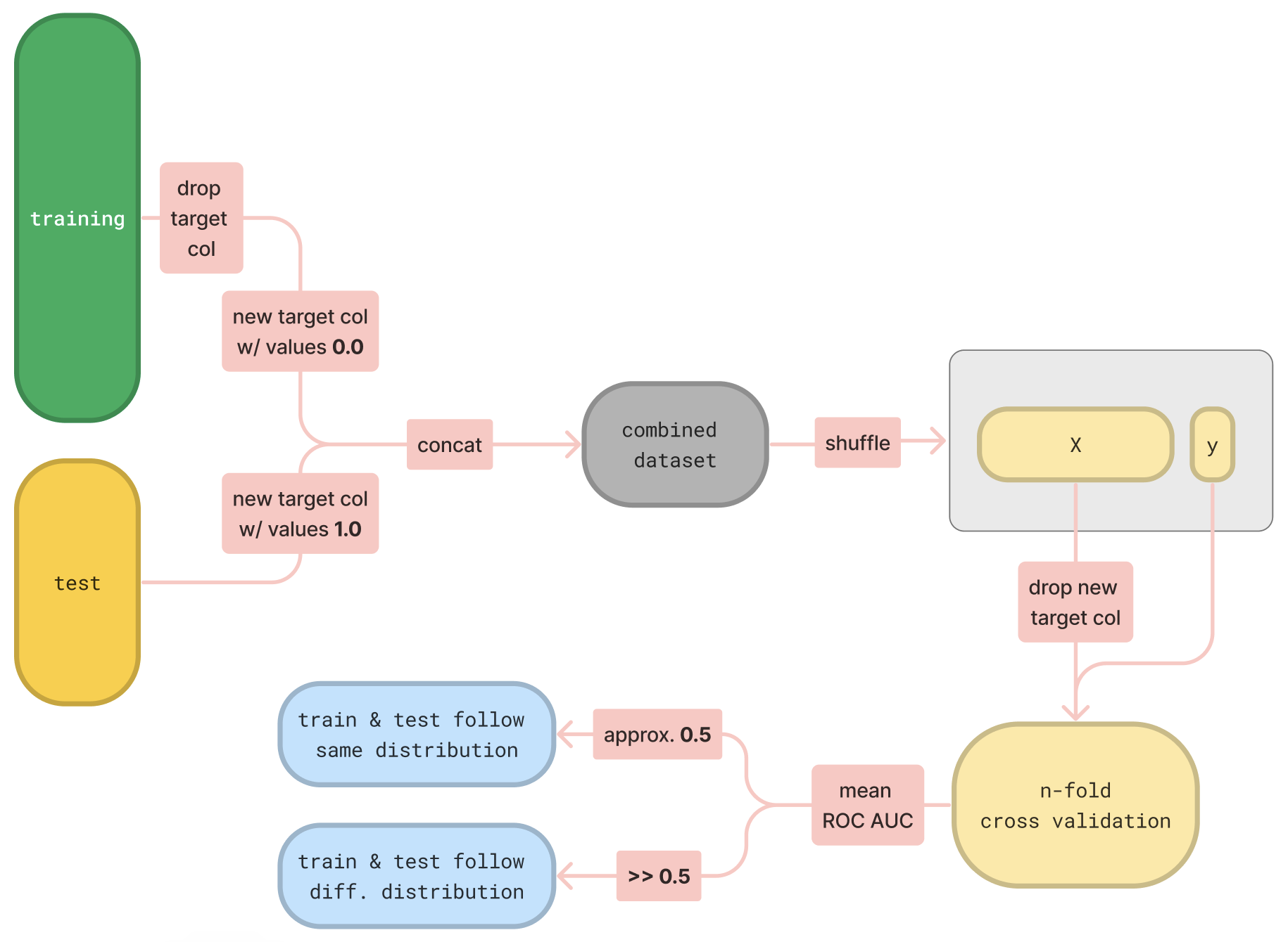
To summarize and formalize the process shown in the video:

1. Combine Datasets: Take your training dataset and your test/production dataset.
2. Create a New Target: Discard the original target variable. Create a new binary target. Assign a value of 0 to all samples from the training set and 1 to all samples from the test set.
3. Train a Classifier: Train a binary classification model (a fast gradient boosting model like LightGBM or CatBoost is an excellent choice) on this new, combined dataset. The model's task is to predict whether a sample belongs to the training set (0) or the test set (1).
4. Evaluate the Classifier: Evaluate your classifier's performance using the ROC AUC score.

The interpretation of the AUC score is the key to quantifying the drift:

• AUC ≈ 0.5: The classifier is performing no better than random chance. This is good news. It means the model cannot distinguish between the train and test sets, suggesting their feature distributions are very similar.
• AUC > 0.7 (and especially approaching 1.0): The classifier is effective at separating the datasets. This is a red flag. It indicates significant distribution drift between your train and test sets. The higher the AUC, the more severe the drift.

This entire workflow is visualized in the diagram below.

Diagnosing the Cause and Taking Action

Simply knowing that drift exists isn't enough. We need to diagnose which features are causing it. The adversarial classifier itself gives us the answer. The feature importances of the trained adversarial model tell us exactly which features were most useful for discriminating between the training and test sets. These are our drifted features.

The following video provides an excellent practical walkthrough of this diagnostic and iterative remediation process.

As the video demonstrates, the process becomes an iterative loop:

1. Run adversarial validation.
2. If AUC is high, inspect the feature importances of the adversarial model.
3. Analyze the top-drifting features. Is the drift expected (e.g., a timestamp)? Is it problematic?
4. Decide on a remediation strategy:
   • Remove the feature: If it's not critical or is a source of leakage (like a record ID that increments over time).
   • Transform the feature: As shown in the video, transform Firefox 61.0 to just Firefox to make it more stable over time. You might transform absolute timestamps into relative features like days_since_release.
   • Do nothing and accept it: If the drift is a natural and important evolution of your data (e.g., financial time series), you might not remove the feature. Instead, the high AUC score informs you that a simple random train-test split is invalid and you must use a time-based split (e.g., train on older data, validate on newer data).
5. Re-run adversarial validation to confirm that the AUC has decreased.

This iterative process is a powerful debugging and feature engineering tool.

Advanced Application: Creating a Robust Validation Set

Adversarial validation has applications beyond just feature removal. In many scenarios, particularly with time-series data, a standard K-fold cross-validation is flawed because it assumes data is IID (Independent and Identically Distributed). Adversarial validation can help us build a more realistic validation set.

This is a more advanced technique, often seen in competitive machine learning and sophisticated production systems.

The key idea from the paper is to use the adversarial classifier not for its feature importances, but for its predictions. The samples in the training set that the classifier assigns a high probability of being from the test set are the ones most similar to your test data. By creating a validation set from these specific samples, you get a much more accurate estimate of how your model will perform on the actual test data. This is crucial in MLOps for reliable model evaluation before deployment.

Interview & Business Context Alert

Question: "You've deployed a model, and after three months, its performance has dropped by 15%. Your monitoring dashboards show no data outages or major schema changes. How would you diagnose this 'silent killer'?"

Your Analysis: "My primary hypothesis would be distribution drift. To confirm this, I would immediately apply adversarial validation.

1. Data Sampling: I'd take the original dataset used for training and a representative sample of production data from the last month.
2. Adversarial Setup: I would combine these datasets, create a binary target where 0 is the original training data and 1 is the recent production data, and train a LightGBM classifier to distinguish between them.
3. Diagnosis & Quantification: I'd evaluate the ROC AUC of this classifier.
   • If the AUC is high, say 0.90, it confirms significant drift and quantifies its severity.
   • I would then inspect the classifier's feature importances. This would give me a ranked list of the features whose distributions have shifted the most between the training period and now.
4. Action Plan: The specific drifted features would guide my next steps. For example, if a feature like user_device_model is at the top of the list, it might indicate a flood of new device types in our user base. The action could be to retrain our main model on more recent data that includes these new devices. If a time-based feature is the cause, it would confirm that our model is stale and a retraining cadence needs to be established. This data-driven diagnosis is far more efficient than guessing."

Conclusion

Adversarial validation is a versatile and essential technique in the modern ML practitioner's toolkit. It moves beyond simple train/test splits and forces us to confront the reality of changing data distributions.

Key Takeaways:

• Distribution drift is a common cause of model performance degradation in production.
• Adversarial validation reframes drift detection as a simple binary classification problem, where the goal is to distinguish between training and test/production data.
• The ROC AUC of the adversarial classifier quantifies the degree of drift.
• The feature importances of the adversarial classifier diagnose the source of the drift, pointing you to the specific features that have changed.
• This technique can be used not only to debug and select features but also to create more robust and representative validation sets.

What's Next?

We've now covered several advanced principles, from strategic design to the validation technique we explored today. The final lesson in this module will synthesize this knowledge. We will zoom back out and learn to explain common system design interview questions related to feature engineering pipelines and their expected answers. This will help solidify the concepts from this module and prepare you to articulate your strategic thinking in a professional setting.