Interpreting Loss Curves for Overfitting and Underfitting

Introduction

In our last lesson, we assembled the complete machinery of a neural network, building a training loop that iteratively refines its parameters through gradient descent. We now have a model that can learn. However, the ability to learn is not the same as the ability to generalize. A model that perfectly memorizes the license plates of cars in its training data is useless for identifying cars it has never seen before.

This lesson transitions us from being builders to being diagnosticians. We will explore how to monitor a model's learning process to determine not just if it's learning, but how well it's generalizing. To do this, we must first split our data into distinct sets:

• Training Set: The data the model learns from. The gradients are computed based on the loss on this set.
• Validation Set: A separate portion of data that the model does not train on. We use it to evaluate the model's performance on unseen data during training, helping us tune hyperparameters and diagnose issues.
• Test Set: A final, held-out set of data that is used only once, after all training and validation is complete, to provide an unbiased estimate of the model's performance in the real world.

By plotting the model's performance on both the training and validation sets over time, we can generate training curves. These plots are the ECGs of machine learning, allowing us to diagnose two of the most fundamental problems in the field: overfitting and underfitting.

The Theoretical Root: The Bias-Variance Tradeoff

Before we look at the curves themselves, we must understand the theoretical tension they represent. The total error of a model can be conceptually decomposed. For a regression problem using Mean Squared Error, this decomposition is precise:

Let's ground these terms in intuition:

• Bias is the error introduced by the model's simplifying assumptions. A model with high bias is too simple and fails to capture the underlying complexity of the data. This leads to underfitting. Think of trying to model a sine wave with a straight line; the linear model is inherently biased and will be wrong no matter how much data you give it.
• Variance is the model's sensitivity to the specific training data it was given. A model with high variance is too complex and fits the noise in the training data, not just the signal. This leads to overfitting. Think of fitting a 20th-degree polynomial to 21 noisy data points; it will pass through them perfectly but will oscillate wildly and perform terribly on any new points.
• Irreducible Error (${\sigma }^2$) is the inherent noise in the data itself, which no model can eliminate.

The "tradeoff" arises because actions taken to decrease bias (e.g., increasing model complexity) often increase variance, and vice versa. Our goal is to find a "sweet spot" that minimizes the total error.

To explore this foundational concept, we'll turn to a classic lecture from Caltech's Yaser Abu-Mostafa, which provides a rigorous yet intuitive explanation.

With this theoretical grounding, we can now interpret the patterns we see in practice.

The Diagnostic Tool: Reading the Curves

When we train a neural network, we typically monitor the loss and/or accuracy on both the training and validation sets at the end of each epoch. The resulting plots reveal the model's behavior.

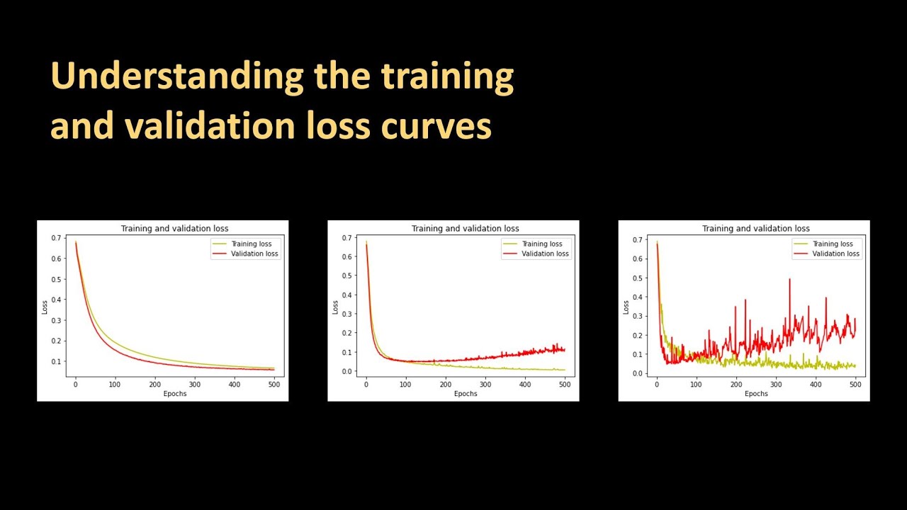
Let's use a practical video guide to understand how to interpret these curves for models of varying complexity.

Let's formalize these visual patterns.

Diagnosis 1: Underfitting (High Bias)

An underfitting model is not complex enough to capture the patterns in the data.

• The Signature: Both the training and validation loss are high and plateau at a similar, suboptimal value. The model isn't performing well even on the data it was trained on.
• What it means: Your model's architecture is fundamentally too simple for the task. From a systems perspective, you've provided an under-powered engine.
• What to do:
  1. Increase Model Complexity: Add more layers or more neurons per layer.
  2. Engineer Better Features: Provide the model with more informative inputs.
  3. Reduce Regularization: If you are using techniques that penalize complexity (which we'll cover next lesson), you may be constraining the model too much.
  4. Train Longer: If the curves haven't flattened out, the model might just need more iterations to converge.

A common and costly mistake is to try and fix underfitting by collecting more data. If the model is too simple, more data will not help it learn a pattern it is incapable of representing.

Diagnosis 2: Overfitting (High Variance)

An overfitting model is too complex for the amount of data available. It has started to memorize the training set, including its noise.

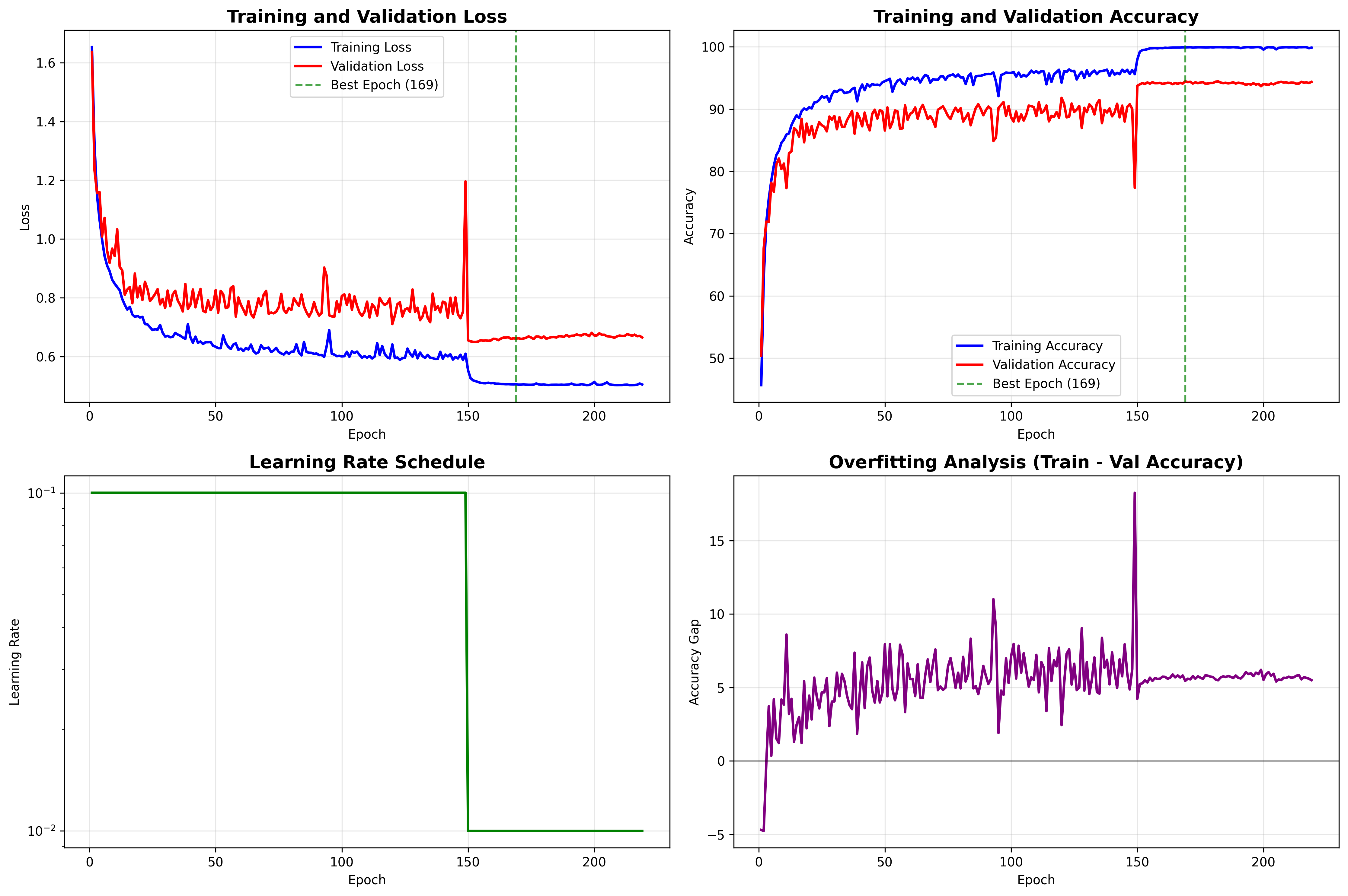
• The Signature: The training loss continues to decrease, while the validation loss stagnates or begins to increase. A significant gap opens up between the two curves.
• What it means: The model is an excellent memorizer but a poor generalizer. It has fit the idiosyncrasies of the training set so well that its performance on new data suffers.
• What to do:
  1. Get More Data: This is the most effective remedy. A more complex model needs more data to learn to generalize properly.
  2. Apply Regularization: Use techniques like L2 regularization (weight decay) or Dropout to penalize model complexity. This is the main topic of our next lesson.
  3. Use a Simpler Model: Reduce the number of layers or neurons.
  4. Data Augmentation: Artificially increase the size of your training set by creating modified copies of your existing data (e.g., rotating or cropping images).
  5. Early Stopping: Stop training at the point where the validation loss is at its minimum, before it starts to rise. In the image below, this would be around epoch 169.

Learning Curves: Will More Data Help?

The training curves we've discussed plot performance against epochs. A related, and arguably more powerful, diagnostic tool is the learning curve, which plots performance against training set size.

The key insight from learning curves is this:

• If your model is high bias (underfitting), the curves will converge to a high error rate quickly. Adding more data will not lower this error. Don't waste time on data collection; you must increase model complexity.
• If your model is high variance (overfitting), there will be a large gap between the training and validation curves. As you add more data, this gap will shrink. This is the primary scenario where collecting more data is the correct solution.

Conclusion

You are now equipped with the essential diagnostic tools for training neural networks. By observing the training and validation curves, you can look "under the hood" of the learning process and understand the behavior of your model.

Key Takeaways:

• Model error is a combination of bias (underfitting) and variance (overfitting).
• Training curves (performance vs. epochs) are the primary tool for diagnosing these issues in a single training run.
  • Underfitting: High training and validation loss; curves converge at a poor value.
  • Overfitting: Low training loss but high validation loss; a large gap appears between the curves.
• A well-fit model shows both training and validation loss converging to a low value with a minimal gap.
• Learning curves (performance vs. dataset size) are the definitive tool to answer the question: "Will more data help?"

Preview of the Next Lesson:

We've spent this lesson diagnosing overfitting, the most common ailment of deep neural networks. In our next lesson, we will focus on the cure. We'll dive into the mathematical and practical implementations of two of the most powerful regularization techniques: L2 Regularization (Weight Decay) and Dropout. We will also explore other critical components for stable training, such as Batch Normalization and intelligent weight initialization schemes.