Building a Training Loop: From Gradients to Optimization

Introduction

In our last lesson, we constructed the core engine of our neural network: the forward_prop and back_prop functions. We now have a mechanism to take an input, generate a prediction, and, most importantly, calculate the precise gradient of the loss function with respect to every single weight and bias in the network. These gradients represent the direction of steepest ascent on the loss surface. However, having a map of the mountain doesn't get us to the valley; we still need to take the steps.

This lesson is about putting that engine into motion. We will construct the full training loop, the iterative process that uses the computed gradients to systematically update the network's parameters, causing it to "learn" from data. We will implement the principle of gradient descent and see how a simple update rule, repeated thousands of times, allows the model to progressively minimize its error and improve its predictions. By the end of this lesson, you will have a complete, trainable neural network, built entirely from first principles.

The Heart of Optimization: Gradient Descent

The entire goal of training is to find the set of parameters (weights $\mathbf{W}$ and biases $\mathbf{b}$) that minimizes our loss function $\mathcal{L}$. From calculus, we know that the gradient, $\nabla \mathcal{L}$, points in the direction of the greatest increase of the function $\mathcal{L}$. Therefore, to minimize the loss, we should take a step in the opposite direction of the gradient.

This is the core idea of gradient descent. We start with a random set of parameters and iteratively update them by moving them "downhill" on the loss surface. The update rule for any single parameter $\theta$ (which can be a weight or a bias) is remarkably simple:

Let's break this down:

• ${\theta }_{\text{old}}$ is the parameter's current value.
• $\frac{\partial \mathcal{L}}{\partial \theta }$ is the gradient of the loss with respect to that parameter, which we get from our back_prop function.
• $\eta$ (eta) is the learning rate, a small positive scalar that controls the size of our update step.

The choice of learning rate is one of the most critical hyperparameters in training a neural network.

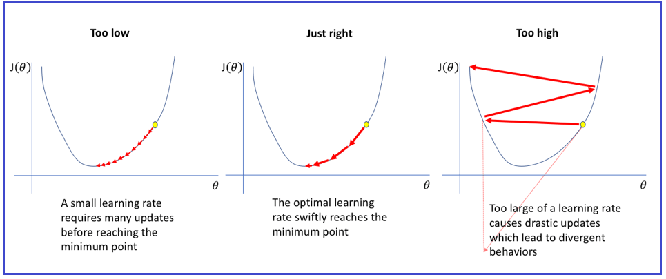
This diagram illustrates how the learning rate affects gradient descent. A rate that is too low leads to slow convergence. A rate that is too high can cause the updates to overshoot the minimum and diverge. An optimal rate converges efficiently.

Your experience with performance systems might suggest an analogy here: think of the learning rate as the time step in a physics simulation. Too large a step, and the simulation becomes unstable and explodes. Too small, and it takes an impractically long time to see any significant change.

Implementing the Training Loop

A full training cycle, or epoch, involves passing the entire dataset through the network, calculating gradients, and updating the parameters. In practice, especially with large datasets, we often update parameters after processing smaller batches of data (Stochastic Gradient Descent or Mini-batch Gradient Descent). For our current from-scratch implementation, we'll stick to batch gradient descent, where we process all training examples at once.

The training process can be broken down into a loop with four main steps:

1. Initialize Parameters: Start with random weights and biases.
2. Forward Pass: Compute the model's predictions and cache intermediate values.
3. Backward Pass: Compute the gradients of the loss with respect to all parameters.
4. Update Parameters: Adjust the parameters using the gradients and the learning rate.
5. Repeat for many iterations.

We've already implemented steps 2 and 3. Now let's implement step 4 and assemble the full loop.

The core of the gradient_descent function looks like this:

# 1. Initialize parameters
W1, b1, W2, b2 = init_params()

# Loop for a specified number of iterations
for i in range(iterations):
    # 2. Forward pass
    Z1, A1, Z2, A2 = forward_prop(W1, b1, W2, b2, X)
    
    # 3. Backward pass
    dW1, db1, dW2, db2 = back_prop(Z1, A1, Z2, A2, W2, X, Y)
    
    # 4. Update parameters
    W1, b1, W2, b2 = update_params(W1, b1, W2, b2, dW1, db1, dW2, db2, alpha)
    
    # Periodically print progress
    if i % 10 == 0:
        print("Iteration:", i)
        print("Accuracy:", get_accuracy(get_predictions(A2), Y))

Here, alpha is the variable name used for the learning rate $\eta$. This loop elegantly combines the components we've built into a machine that learns. With each iteration, the parameters W1, b1, W2, b2 are nudged in a direction that reduces the error, and the accuracy should steadily climb.

From a Script to a System: The Optimizer Abstraction

Our current implementation, while functional, mixes the parameter update logic directly into the training loop. In a large-scale system, this is not ideal. What if we want to switch from simple gradient descent to a more advanced algorithm like Adam? We would have to rewrite the update step.

A more robust, systems-oriented approach is to encapsulate the update logic into an Optimizer class. This aligns with your interest in low-level systems design, where modularity and clear interfaces are paramount. The optimizer's job is to take the parameters and their corresponding gradients and handle the update.

This is exactly how professional deep learning libraries are designed. Let's examine a C++ implementation to see this principle in action.

This object-oriented design is powerful. The training loop doesn't need to know how the parameters are updated, only that it needs to call the optimizer's train or step method. This makes the code more modular, readable, and extensible—key principles in building performant and maintainable systems.

Conclusion

Today, you have closed the loop on the learning process. By combining the forward and backward passes within an iterative gradient descent framework, you have built a complete, working neural network from scratch. You've witnessed how a simple update rule, applied repeatedly, allows a model to learn complex patterns from data.

Key Takeaways:

• The core of training is the training loop, which iteratively performs a forward pass, a backward pass, and a parameter update.
• Gradient Descent is the fundamental optimization algorithm that updates parameters by taking steps in the opposite direction of the loss gradient.
• The learning rate ($\eta$) is a critical hyperparameter that controls the step size of the updates.
• Encapsulating the update logic in an Optimizer class is a key software engineering principle that makes training code modular and scalable, as seen in both high-level Python libraries and low-level C++ implementations.

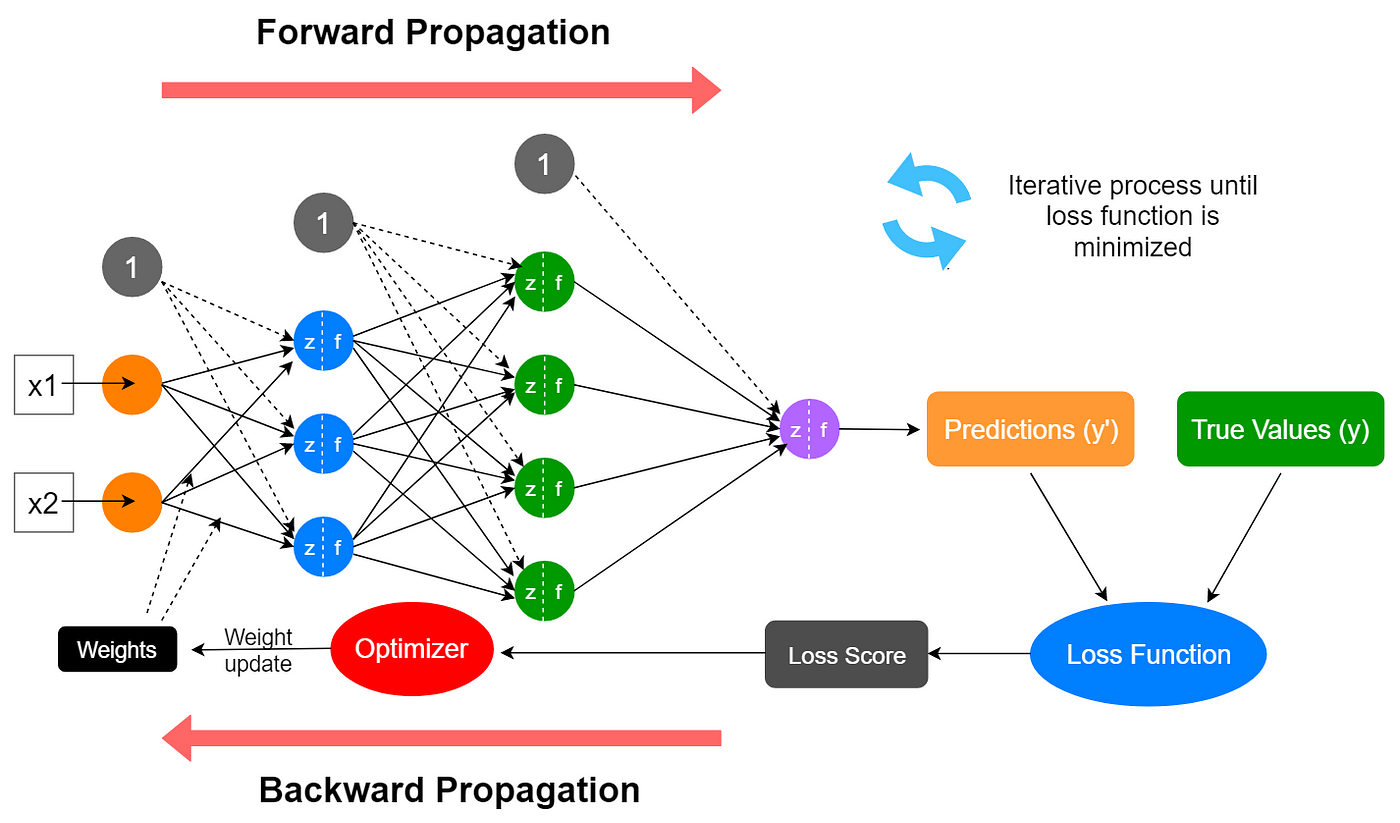
This diagram provides a complete overview of the process we have now implemented. Data flows forward to make predictions, a loss is calculated, and the error signal flows backward to compute gradients, which an optimizer uses to update the weights.

Preview of the Next Lesson:

Our network can now learn, but how well is it learning? Is it memorizing the training data, or is it truly generalizing? In the next lesson, we will become detectives. We will learn how to diagnose the health of our training process by analyzing training and validation curves to spot overfitting and underfitting. We will then explore fundamental techniques like regularization to combat these issues and build more robust models.