L2 Regularization: Derivation and Effect on Model Parameters

Recommended resources

The freely available resources this lesson will direct you to.

Introduction

In our previous lesson, we developed the diagnostic skills to identify overfitting by analyzing training and validation curves. We saw that when a model has too much capacity for the given data (high variance), it begins to memorize noise, causing validation loss to stagnate or rise while training loss plummets. We are now moving from diagnosis to treatment.

This lesson introduces our first and perhaps most fundamental regularization technique: L2 Regularization, also known as Weight Decay. We will derive this method from first principles, connect it to its classical machine learning ancestor, and understand precisely how it combats overfitting by constraining the values of a model's parameters. Our goal is to understand not just what weight decay does, but why it works, from both an optimization and a probabilistic perspective.

The Problem with Large Weights

Overfitting often manifests as a model learning an excessively complex, "spiky" function to perfectly accommodate every training point, including the noise. From a mathematical standpoint, creating sharp, localized changes in a function's output requires its parameters—the weights—to take on large absolute values. A simple, smooth function, by contrast, tends to have smaller, more evenly distributed weights.

This gives us a clear strategy: if large weights enable overfitting, we can discourage them by penalizing the model for having large weights. We can modify our optimization objective from simply minimizing the data loss to minimizing the data loss plus a penalty for the "size" of the weight vector $w$ .

Formulating the Penalty: L2 Regularization

To penalize the size of the weight vector, we need a way to measure it. In Module 1, we introduced vector norms as a way to quantify vector magnitude. The most common choice for regularization is the squared L2 norm, $∥ w ∥_{2}^{2}$ .

We add this penalty to our original loss function $L_{data}$ , creating a new objective function $J (w, b)$ :

J (w, b) = L_{data} (w, b) + \frac{λ}{2} ∥ w ∥_{2}^{2}

Let's break this down:

$∥ w ∥_{2}^{2} = \sum_{j} w_{j}^{2}$ : This is the squared Euclidean norm of the weight vector. We use the square for computational convenience; it removes the square root and makes the derivative much simpler, which you'll appreciate when we derive the update rule.
$λ$ : The regularization parameter is a non-negative hyperparameter. It controls the strength of the penalty.
- If $λ = 0$ , we recover the original loss function with no regularization.
- As $λ \to \infty$ , the penalty on the weights dominates, forcing them toward zero regardless of the data loss.
The $\frac{1}{2}$ is a convention that simplifies the derivative, as the power of 2 from the squared term will cancel it out.

Note that we typically only regularize the weights $w$ and not the bias terms $b$ . A large bias doesn't affect the model's complexity in the same way as large weights; it merely shifts the output, and there are far fewer bias terms than weights.

To solidify this foundational concept, the following reading from the Dive into Deep Learning book formally introduces the L2 penalty.

3.7. Weight Decay

This section from Dive into Deep Learning formally introduces the motivation for penalizing model complexity and defines the L2-regularized loss function.

Please read the text starting from this section. As you read, focus on the rationale for choosing the L2 norm and the role of the hyperparameter \lambda. The text also briefly contrasts L2 with L1 regularization (Lasso), which is useful context.

The Classical Bridge: Constrained Optimization and Ridge Regression

Before this technique was applied to deep learning, L2 regularization was a cornerstone of classical statistics, where L2-regularized linear regression is known as Ridge Regression.

We can view this problem from a different angle: instead of adding a penalty term, we can formulate it as a constrained optimization problem. The goal is to minimize the original data loss $L_{data} (w)$ subject to the constraint that the size of the weight vector does not exceed a certain threshold, $t$ :

w min L_{data} (w) subject to ∥ w ∥_{2}^{2} \leq t

This formulation is equivalent to the one with the $λ$ penalty. $λ$ is mathematically related to the constraint radius $t$ via the method of Lagrange multipliers, a powerful tool from multivariable calculus for solving constrained optimization problems.

This perspective gives us a powerful geometric intuition. Imagine the loss function as a set of elliptical contour lines in the parameter space. The L2 constraint $∥ w ∥_{2}^{2} \leq t$ defines a spherical region (a circle in 2D) centered at the origin. The optimal solution is the point on the lowest possible loss contour that still touches this spherical region.

Geometric interpretation of regularization. The ellipses are contours of the least-squares error. The solution is the point where the ellipse first touches the constraint region (blue). For L2/Ridge Regression (right), the constraint is a circle, pulling the solution towards the origin without necessarily making it sparse. For L1/Lasso (left), the diamond-shaped constraint encourages solutions where some parameters are exactly zero.

This connection between regularization and classical optimization methods is profound. The following video beautifully connects the Lagrange multiplier method you may know from physics to its application in machine learning.

The Lagrange Multiplier “Method” of Machine Learning [Regularization]

This video from CompuFlair, "The Lagrange Multiplier 'Method' of Machine Learning," provides a deep connection between the physics concept of constrained optimization and regularization in ML.

First, watch the section from this segment which introduces the probabilistic foundation of regularization. This provides a sneak peek into the Bayesian interpretation which we will touch on later. Next, focus on the core connection from this part. It explicitly frames L2 regularization as minimizing a loss function subject to a spherical constraint, solved via Lagrange multipliers, and introduces the term "Ridge Regression."

Deriving Weight Decay

Now for the central part of our lesson: deriving how this modified loss function changes the gradient descent update rule. This will reveal why L2 regularization is called weight decay.

Our standard gradient descent update rule is:

w_{t + 1} \leftarrow w_{t} - η \nabla_{w} J (w_{t}, b_{t})

where $η$ is the learning rate.

We need to compute the gradient of our new loss function, $J (w, b) = L_{data} (w, b) + \frac{λ}{2} ∥ w ∥_{2}^{2}$ . Using the sum rule for derivatives:

\nabla_{w} J (w, b) = \nabla_{w} L_{data} (w, b) + \nabla_{w} (\frac{λ}{2} ∥ w ∥_{2}^{2})

Let's focus on the new penalty term. Since $∥ w ∥_{2}^{2} = w_{1}^{2} + w_{2}^{2} + \dots + w_{n}^{2}$ , the partial derivative with respect to a single weight $w_{j}$ is:

\frac{\partial}{\partial w _{j}} (\frac{λ}{2} k = 1 \sum n w_{k}^{2}) = \frac{λ}{2} (2 w_{j}) = λ w_{j}

Therefore, the gradient of the penalty term with respect to the entire weight vector $w$ is simply $λ w$ .

Substituting this back, the full gradient is:

\nabla_{w} J (w, b) = \nabla_{w} L_{data} (w, b) + λ w

Now, let's plug this into our gradient descent update rule:

w_{t + 1} \leftarrow w_{t} - η (\nabla_{w} L_{data} (w_{t}, b_{t}) + λ w_{t})

Here comes the crucial step. Let's rearrange the terms to isolate the effect on $w_{t}$ :

w_{t + 1} \leftarrow w_{t} - η λ w_{t} - η \nabla_{w} L_{data} (w_{t}, b_{t})

w_{t + 1} \leftarrow (1 - η λ) w_{t} - η \nabla_{w} L_{data} (w_{t}, b_{t})

This final equation reveals the mechanism of weight decay. Before performing the standard gradient update based on the data loss, we first multiply the current weights $w_{t}$ by a factor of $(1 - η λ)$ . Since $η$ and $λ$ are small positive numbers, this factor is slightly less than 1. This means that at every single update step, the weights are first shrunk, or decayed, towards zero.

The following resources will walk you through this derivation and its practical consequences.

3.7. Weight Decay

This section of the Dive into Deep Learning text provides the precise update equation we just derived.

Please read the short section containing the equation, starting from this paragraph. This will reinforce the mathematical form of the weight decay update.

NN - 16 - L2 Regularization / Weight Decay (Theory + @PyTorch code)

This video by Meerkat Statistics provides an excellent and concise theoretical explanation of L2 regularization and weight decay.

First, watch the introduction from the beginning, which defines the L2 regularized loss function. Next, follow the derivation from this segment. The presenter derives the exact same weight decay update rule we did and provides a nice analogy to a continuous-time differential equation, showing the weights decay exponentially.

The Effect in Practice

The consequence of this decay is a smoother, less complex model that generalizes better. The regularization term forces the optimizer to find a balance between fitting the training data and keeping the weights small.

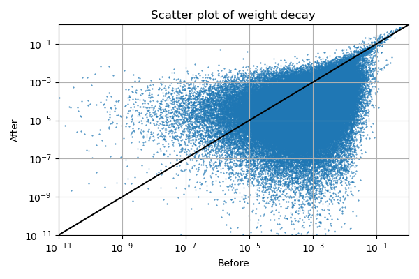
A scatter plot showing the magnitude of weights before and after training with weight decay. Each point represents a single weight. The x-axis is its magnitude before decay, and the y-axis is its magnitude after. Points below the black line (y=x) have been shrunk, illustrating the decay effect across the entire network.

The Meerkat Statistics video also provides a powerful visual and a practical demonstration in PyTorch.

NN - 16 - L2 Regularization / Weight Decay (Theory + @PyTorch code)

This video continues to show the intuitive effect of L2 regularization and how to implement it in PyTorch.

Watch the segment from this part for the intuition. You'll see how a model trained on a noisy sine wave produces a "crazy" overfitted function without regularization, and a much smoother, more general function with it. Finally, see how it's done in practice from the coding section. Notice that while you can add the penalty term to the loss manually, all modern optimizers (like Adam) have a built-in weight_decay parameter that handles it for you. This is the standard way to apply L2 regularization.

A Deeper View: The Probabilistic Perspective

For an even deeper understanding that aligns with your interest in first principles, we can interpret L2 regularization from a probabilistic standpoint using Maximum A Posteriori (MAP) estimation.

Recall from our probability module that Bayes' theorem allows us to find the posterior probability of our parameters given the data:

P (w ∣ Data) \propto P (Data ∣ w) P (w)

$P (Data ∣ w)$ is the likelihood, which is what we maximize in standard Maximum Likelihood Estimation (MLE). Minimizing squared error is equivalent to maximizing a Gaussian likelihood.
$P (w)$ is the prior, our belief about the parameters before seeing any data.

Adding an L2 penalty term to the loss function is mathematically equivalent to placing a Gaussian prior with a mean of zero on the weights $w$ . A zero-mean Gaussian distribution states that weights are most likely to be close to zero and become exponentially less likely as their magnitude increases. When we then optimize the new objective, we are no longer just maximizing the likelihood; we are finding the MAP estimate that balances fitting the data with our prior belief that weights should be small.

This is a beautiful unification of optimization and probabilistic modeling.

Understanding L1 and L2 regularization with analytical and ...

This article provides another perspective on the probabilistic view of L2 regularization.

First, quickly review the definition of L2 regularization in the section L2 regularization. Then, read the section Probabilistic derivation of L2 regularization. This will explicitly show how assuming a Gaussian prior leads directly to the L2 penalty term when you take the negative log of the posterior.

Conclusion

In this lesson, we have taken a deep dive into L2 regularization, or weight decay. We have gone from the high-level intuition of penalizing model complexity to the precise mathematical derivation of the weight decay update rule.

Key Takeaways:

Objective: L2 regularization combats overfitting by adding a penalty term, $\frac{λ}{2} ∥ w ∥_{2}^{2}$ , to the loss function.
Mechanism: In gradient descent, this penalty term results in an update rule that first shrinks weights by a factor of $(1 - η λ)$ before applying the data-based gradient update. This is why it's called weight decay.
Geometric View: It's equivalent to solving a constrained optimization problem (Ridge Regression) where the loss is minimized within a spherical region in parameter space.
Probabilistic View: It is equivalent to performing MAP estimation with a zero-mean Gaussian prior on the model's weights, encoding a "belief" that smaller weights are more likely.
Effect: The result is a simpler, smoother model with smaller weights, which is less sensitive to noise in the training data and generalizes better to unseen data.

Preview of the Next Lesson:

Weight decay constrains the values of the parameters. Next, we will explore two other powerful techniques that work in fundamentally different ways. Dropout is a regularization method that randomly deactivates neurons during training, forcing the network to learn more robust and redundant features. Batch Normalization is a technique that normalizes the activations within the network, which has a slight regularizing effect but is primarily used to stabilize and accelerate the training of very deep networks.