Dropout and Batch Normalization: Mechanisms and Roles

Introduction

In our last lesson, we explored L2 regularization, a technique that combats overfitting by penalizing the magnitude of a model's weights. This encourages the network to learn smoother, simpler functions. We saw how this penalty term leads directly to the "weight decay" update rule, where weights are multiplicatively shrunk at each training step.

Today, we shift our focus from controlling parameter values to two powerful techniques that manipulate the network in entirely different ways. We will investigate Dropout, which regularizes by altering the network's architecture at every step, and Batch Normalization, which stabilizes training by transforming the data as it flows between layers. While they have different primary goals—regularization vs. stabilization—both have become indispensable tools for training modern deep neural networks.

Our objective is to understand the precise mechanisms behind each technique, from their mathematical formulation to their practical implementation, and to clarify their distinct roles in building robust and efficient models.

Part 1: Dropout - Regularization by Randomness

In a large, complex network, it's possible for groups of neurons to "co-adapt," meaning they become highly reliant on each other to correct mistakes. This can lead to the network memorizing noise, as these specialized neuron cliques may not generalize well to unseen data.

Dropout offers a radical solution: what if we prevent neurons from reliably co-adapting by making their presence unpredictable?

The core idea of Dropout is to randomly set the outputs of some neurons to zero during each forward pass of the training phase. This has two profound effects:

1. It forces each neuron to learn more robust features that are useful on their own, without relying on specific other neurons being active.
2. It's akin to training an ensemble of many different, smaller neural networks. Since a different set of neurons is dropped at each step, we are implicitly averaging over an exponential number of thinned architectures.

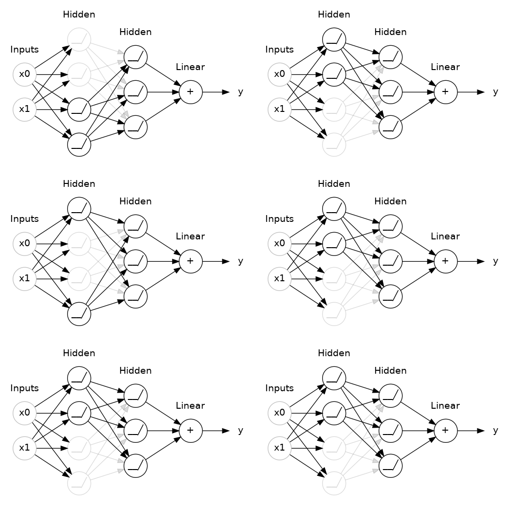
The Mechanism of Inverted Dropout

A naive implementation of Dropout would simply zero-out neurons during training. However, this would create a mismatch between training and testing. At test time, all neurons are active, so the total input to the next layer would be significantly larger than it was during training.

To solve this, we use a technique called inverted dropout. During training, after zeroing out the dropped neurons, we scale up the activations of the remaining "active" neurons by the inverse of the probability of keeping a neuron.

Let's formalize this. Suppose we want to apply Dropout to a layer's activation vector $\mathbf{a}$ with a keep_prob of $p$.

1. Create a Mask: We generate a binary mask vector $\mathbf{d}$ of the same shape as $\mathbf{a}$, where each element is drawn from a Bernoulli distribution, $d_i\sim \text{Bernoulli}(p)$. Each element of $\mathbf{d}$ is 1 with probability $p$ and 0 with probability $1-p$.

2. Apply the Mask: We perform element-wise multiplication to drop neurons: ${\mathbf{a}}_{\text{dropped}}=\mathbf{a}\odot \mathbf{d}$.

3. Scale (Invert): We scale the result to maintain the expected output magnitude: ${\mathbf{a}}_{\text{final}}=\frac{{\mathbf{a}}_{\text{dropped}}}{p}$.

This scaling ensures that the expected value of the layer's output is the same during training and testing. At test time, we simply use the full network without any dropout or scaling, making inference computationally identical to a standard network.

During backpropagation, the gradient is only passed through the neurons that were active (where the mask $\mathbf{d}$ was 1). The scaling factor $\frac{1}{p}$ is also applied to the gradient to ensure the updates are of the correct magnitude.

The following video provides an excellent and complete walkthrough of Dropout, from the core intuition to a from-scratch Python implementation.

Part 2: Batch Normalization - Stabilizing a Moving Target

As a network trains, the weights in the early layers are constantly updated. This causes the distribution of activations fed into later layers to continuously change—a problem known as Internal Covariate Shift. Each layer is trying to learn from a non-stationary input distribution, which is like trying to hit a moving target. This can destabilize training, forcing us to use lower learning rates and be very careful with weight initialization.

Batch Normalization (BN) addresses this problem by explicitly normalizing the inputs to each layer for every mini-batch.

The Mechanism of Batch Normalization

For a mini-batch of $m$ examples, BN transforms the activations for each feature independently. The process consists of two main steps:

1. Normalization:

   • First, calculate the mean ${\mu }_{\mathcal{B}}$ and variance ${\sigma }_{\mathcal{B}}^2$ of the activations for a specific feature across the current mini-batch $\mathcal{B}$.
   $${\mu }_{\mathcal{B}}=\frac{1}{m}\sum _{i=1}^m{x}_i$$ $${\sigma }_{\mathcal{B}}^2=\frac{1}{m}\sum _{i=1}^m(x_i-{\mu }_{\mathcal{B}}{)}^2$$
   • Then, normalize each activation $x_i$ to have zero mean and unit variance. An epsilon $ϵ$ is added for numerical stability.
   $${\hat{x}}_i=\frac{x_i-{\mu }_{\mathcal{B}}}{\sqrt{{\sigma }_{\mathcal{B}}^2+ϵ}}$$

2. Scale and Shift:

   • Forcing all layer inputs to have a fixed distribution might be too constraining. For example, for a sigmoid activation, this would force inputs into the linear regime around zero, reducing the network's non-linear capacity.
   • To restore the network's expressive power, BN introduces two new learnable parameters per feature: a scale parameter $\gamma$ and a shift parameter $\beta$. These are updated via gradient descent just like the network's weights.
   $$y_i=\gamma {\hat{x}}_i+\beta$$

   This allows the network to learn the optimal mean and variance for each layer's input. If the network finds it optimal, it can learn $\gamma =\sqrt{{\sigma }_{\mathcal{B}}^2}$ and $\beta ={\mu }_{\mathcal{B}}$ to effectively undo the normalization and recover the original activations.

The following reading provides a concise mathematical summary of these steps.

Backpropagation and Inference

The backward pass through a Batch Normalization layer is more complex than it might first appear. Because the mean and variance are computed across the entire mini-batch, the gradient of the loss with respect to a single input $x_i$ depends on all other inputs $x_j$ in that same batch. This introduces dependencies that span the entire batch.

For a rigorous, first-principles understanding of this gradient flow, the following resource provides an exceptional step-by-step breakdown using a computational graph.

A final critical point is how BN operates at inference time. Since we might be processing a single input, we can't compute a batch mean and variance. The solution is to estimate the population statistics during training.

• During training, the BN layer maintains an exponential moving average of the means (${\mu }_{\text{run}}$) and variances (${\sigma }_{\text{run}}^2$) calculated from each mini-batch.
• At test time, these "frozen" running averages are used in place of batch-specific statistics for normalization. The learned $\gamma$ and $\beta$ are used as usual.

This video expertly explains both the backpropagation derivation and the crucial training vs. inference distinction.

Conclusion

We have now explored two fundamentally different but equally important techniques for training deep networks.

Key Takeaways:

• Dropout is a regularization technique.

  • Mechanism: It randomly sets neuron activations to zero during training and scales the rest using inverted dropout. At test time, it does nothing.
  • Role: It prevents neuron co-adaptation, forcing the network to learn more robust, redundant features and acting as a form of model ensembling.

• Batch Normalization is a training stabilization technique.

  • Mechanism: It normalizes layer inputs per mini-batch to have zero mean and unit variance, then applies a learnable scale ($\gamma$) and shift ($\beta$). It uses moving averages of statistics for inference.
  • Role: It mitigates internal covariate shift, allowing for higher learning rates, faster convergence, and reduced sensitivity to weight initialization. It also has a minor regularizing effect.

Preview of the Next Lesson:

Batch Normalization significantly reduces the network's sensitivity to the scale of its initial weights. However, it doesn't eliminate the need for careful initialization altogether. Poorly chosen initial weights can still lead to issues like vanishing or exploding gradients, especially in very deep networks without BN. In our next lesson, we will investigate this problem from first principles and derive modern weight initialization strategies like Xavier/Glorot and He initialization, which are designed to maintain a stable signal variance as data propagates through the network.