CAN Bus Physical Layer

Hello! Welcome back to our course on advanced automotive diagnostics.

In our first lesson, we mapped the entire diagnostic protocol stack to the OSI model, placing the CAN bus at the foundational Physical (Layer 1) and Data Link (Layer 2) layers. Now, we'll zoom in on Layer 1 to build a solid understanding of the hardware that makes all vehicle communication possible.

This lesson is dedicated to the CAN bus physical layer. We will cover its essential characteristics, including the electrical signaling and the critical role of bus termination. A firm grasp of this layer is indispensable for both software development and system testing. When you're debugging why an ECU won't respond, the physical layer is often the first place to look.

The CAN Bus Topology: A Two-Wire Backbone

At its core, the high-speed CAN bus (as defined by ISO 11898-2) is a linear network, often called a "backbone," that connects various Electronic Control Units (ECUs). This network is built on two wires:

• CAN High (CAN_H)
• CAN Low (CAN_L)

These two wires are typically twisted together, forming a twisted pair. This isn't just for neatness; as we'll see, twisting the wires is a simple but highly effective way to protect the signals from electrical noise, which is abundant in a vehicle.

ECUs are not connected in a star pattern but are instead tapped into this main backbone using short connections called "stubs." The two physical ends of the main backbone must be terminated with resistors.

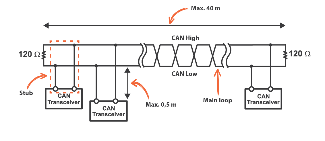
To begin, let's get a clear overview of these physical components and their layout.

Differential Signaling: The Secret to Noise Immunity

You might wonder why CAN uses two wires instead of a single wire referenced to ground. The answer is differential signaling, a technique that makes the CAN bus remarkably robust against the electromagnetic interference (EMI) found in automotive environments (e.g., from ignition systems, electric motors, and radio transmitters).

Instead of measuring the voltage of a single wire relative to ground, a CAN transceiver measures the difference in voltage between the CAN_H and CAN_L lines.

• When noise is induced onto the bus, it typically affects both wires almost equally because they are twisted together and run in close proximity.
• When the receiver subtracts the voltage of CAN_L from CAN_H, this "common-mode" noise is cancelled out, leaving only the intended signal.

This principle not only makes the bus resilient to picking up noise but also reduces the amount of electromagnetic noise the bus emits, preventing it from interfering with other systems.

The following video segment explains this core principle with clear animations.

Bus States and Voltage Levels

The differential signal on the bus creates two distinct logical states:

1. Recessive State (Logic '1'): This is the idle or default state of the bus. In this state, both CAN_H and CAN_L are held at approximately 2.5V. The differential voltage (CAN_H - CAN_L) is therefore close to 0V.
2. Dominant State (Logic '0'): This is the active state used to transmit data bits. A transceiver actively drives the bus into this state by raising CAN_H to about 3.5V and lowering CAN_L to about 1.5V. This creates a differential voltage of approximately 2V.

It is crucial to remember this mapping: a logical '0' is the "dominant" state, and a logical '1' is the "recessive" state. This has important implications for bus arbitration, which we will cover in a later lesson.

As a system tester, you won't always have an oscilloscope handy. The next resource shows what these signals look like on a scope and, more practically, what you can expect to read with a standard multimeter.

Bus Termination: Preventing Signal Reflections

As you've seen, every CAN bus requires two 120-Ohm (Ω) resistors, one at each physical end of the main backbone. These are not optional; the bus will not function reliably without them. They serve two critical purposes.

1. Preventing Signal Reflections

High-speed electrical signals behave like waves. When a signal traveling down a wire reaches the end, it can "reflect" back, like an echo. This reflected signal interferes with subsequent signals, corrupting the data. The termination resistors absorb the signal energy at the ends of the bus, preventing these reflections. The 120Ω value is chosen to match the characteristic impedance of the twisted-pair cable, which ensures maximum energy absorption.

2. Defining the Recessive State

CAN transceivers use an "open-collector" (or more accurately, open-drain) output. This means they can only actively pull the bus into the dominant state. They cannot actively drive it to the recessive state. When all transceivers are "off," the termination resistors serve to pull the CAN_H and CAN_L lines together, returning the bus to the ~2.5V recessive level.

To understand these functions in more detail, let's return to our first video resource.

For a more in-depth technical explanation, you can refer to the document below from Texas Instruments, a major manufacturer of CAN transceivers.

Troubleshooting with Termination Resistance

Because correct termination is so vital, the first step in troubleshooting a CAN bus is often to measure the total resistance. With the network unpowered, you can use a multimeter to measure the resistance between the CAN_H and CAN_L pins at any point on the bus. Since the two 120Ω resistors are at opposite ends of the parallel bus, the total resistance should be:

$R_{total}=\frac{R_1\times R_2}{R_1+R_2}=\frac{120\times 120}{120+120}=60\Omega$

Test your understanding!

You are tasked with troubleshooting a test bench where an ECU is not communicating. You turn off the power to the network and measure the resistance between the CAN_H and CAN_L pins on the ECU's connector. Your multimeter reads 119.8 Ω.

What is the most likely physical layer problem?

Show answer

The most likely problem is that one of the two 120Ω termination resistors is missing from the bus. A reading of ~120Ω indicates that only one terminator is present. A correct reading would be ~60Ω.

The following short clip demonstrates exactly this measurement procedure.

Physical Design Rules

For a CAN bus to be reliable, especially at high data rates (500 kbps, 1 Mbps), some physical design rules must be respected:

• Stub Length: As mentioned, stubs are the short wires connecting an ECU to the main backbone. These stubs also cause minor signal reflections. To keep these reflections from corrupting data, stub lengths must be kept as short as possible. The ISO 11898 standard recommends a maximum stub length of 0.3 meters for a 1 Mbps network. Long stubs are a very common cause of communication errors.
• Bus Length vs. Data Rate: There is an inverse relationship between the maximum possible length of a CAN bus and the data rate. Signal propagation delay becomes a limiting factor over long distances. For example:
  • 1 Mbps: ~40 meters max length
  • 500 kbps: ~100 meters max length
  • 125 kbps: ~500 meters max length
• Grounding: To prevent "ground loops" and common-mode voltage offsets between ECUs, the network should have a single, solid ground reference.

Conclusion

In this lesson, we took a detailed look at the CAN physical layer. You learned about the components and principles that ensure reliable data transmission in the harsh automotive environment.

Key Takeaways:

• Physical Topology: CAN is a linear bus using a twisted pair of wires (CAN_H, CAN_L) with ECUs connected via short stubs.
• Differential Signaling: The bus's key feature for noise immunity. The receiver interprets the voltage difference between CAN_H and CAN_L, canceling out common-mode noise.
• Bus States: The bus operates in two states: recessive (logic '1') with a ~0V differential and dominant (logic '0') with a ~2V differential.
• Termination: Two 120Ω resistors are mandatory, one at each end of the bus. They prevent signal reflections and define the recessive state. Correct termination results in a total bus resistance of 60Ω.
• Design Rules: Reliability depends on adhering to rules for stub length, bus length, and proper grounding.

With this understanding of the physical medium, we are now ready to move up the stack. In our next lesson, we will dissect the structure of the data packets that travel over these wires, exploring the fields within a Classical CAN frame.