Recommended resources
The freely available resources this lesson will direct you to.
Introduction
In our last lesson, we examined the internal architecture of a modern GPU, focusing on the Streaming Multiprocessor (SM) as its fundamental execution engine. We identified key components like CUDA cores for general-purpose math and, crucially for AI, specialized Tensor Cores designed to accelerate matrix operations.
This lesson connects that hardware architecture directly to its primary application: deep learning. Our goal is to answer the question posed by this lesson's learning outcome: Explain why the parallelism and arithmetic intensity of GPUs are well-suited for deep learning workloads. We will explore two core concepts:
- The inherent parallelism of deep learning algorithms: We'll see how the mathematical operations at the heart of neural networks are naturally suited for a SIMT execution model.
- Arithmetic Intensity: We will define this critical performance metric, which measures the ratio of computation to memory access. Using the Roofline Model, we will analyze why the high arithmetic intensity of many deep learning operations is a perfect match for the high compute-to-bandwidth ratio of GPU architectures.
The Parallel Nature of Deep Learning
At its core, deep learning involves performing a series of mathematical operations—primarily matrix multiplications, convolutions, and element-wise functions—on large tensors of data. The key insight is that the vast majority of these computations are independent of one another.
Consider a simple matrix multiplication, . Each element is the dot product of the i-th row of A and the j-th column of B. The calculation of has no dependency on the calculation of or . They can all be computed simultaneously. When you extend this to a mini-batch of data, the parallelism explodes. This property is often called "embarrassingly parallel" because the problem requires little effort to be decomposed into a massive number of independent tasks.
To visualize this, let's watch a brief explanation that uses computer graphics as an example. While the data is different (vertices instead of activations), the principle of applying a single instruction to multiple data points is identical.
How do Graphics Cards Work? Exploring GPU Architecture
The following clip from Branch Education explains the concept of 'embarrassingly parallel' operations and the Single Instruction, Multiple Data (SIMD) model, which is the foundation of the GPU's SIMT approach. This will help build an intuition for why neural network math is a natural fit for the GPU's execution style.
Watch the section from 16:53 to 20:20. Focus on how a single instruction (a transformation) is applied in parallel to millions of different data points (vertices). This is directly analogous to applying a weight matrix to a batch of input vectors in a neural network.
This massive, data-parallel nature of deep learning workloads is the first reason GPUs are so effective. The thousands of cores organized into SMs, all executing threads in lockstep-like warps, provide the perfect hardware substrate for tackling these problems.
Arithmetic Intensity and the Roofline Model
While parallelism is necessary, it's not sufficient. To understand why GPUs are a particularly efficient match, we need to introduce the concept of arithmetic intensity.
An operation's performance on any processor is ultimately limited by one of two things: the speed at which it can perform calculations (compute-bound) or the speed at which it can feed itself data from memory (memory-bound).
Arithmetic Intensity (AI) quantifies this relationship for a given algorithm:
- A high AI workload (e.g., large matrix multiplication) performs many computations for each byte of data it reads from or writes to memory.
- A low AI workload (e.g., adding two vectors) performs very few computations for each byte transferred.
The following document from NVIDIA provides a clear, concise definition of arithmetic intensity and its implications.
GPU Performance Background User's Guide
This guide from the NVIDIA documentation introduces arithmetic intensity and the concept of a processor's 'ops:byte ratio'. This is the theoretical foundation for our discussion.
Please read Section 4, 'Understanding Performance'. It formally defines arithmetic intensity and explains how comparing it to the hardware's capabilities determines whether an operation will be math-limited or memory-limited.
The relationship between a workload's AI and the hardware's capabilities is visually captured by the Roofline Model.
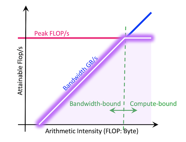
As you saw in the reading, an algorithm is compute-bound if its AI is greater than the processor's ops:byte ratio. GPUs are specifically designed with an extremely high ops:byte ratio—they have immense computational power (TFLOP/s) relative to their memory bandwidth (GB/s). This design choice makes them throughput-oriented machines that excel at workloads with high arithmetic intensity.
Applying the Model to Deep Learning Workloads
Now let's connect the model to real deep learning operations. The NVIDIA document you just read contains a very insightful table.
Table 1. Examples of neural network operations with their arithmetic intensities. (from NVIDIA Docs LINK)
| Operation | Arithmetic Intensity (FLOPS/Byte) | Usually limited by... |
|---|---|---|
| Linear layer (4096 outputs, 1024 inputs, batch size 512) | 315 | arithmetic |
| Linear layer (4096 outputs, 1024 inputs, batch size 1) | 1 | memory |
| Max pooling with 3x3 window and unit stride | 2.25 | memory |
| ReLU activation | 0.25 | memory |
| Layer normalization | < 10 | memory |
This table reveals the critical insight:
- Dot-product operations (linear layers, convolutions), especially when performed on large batches of data, have very high arithmetic intensity. They perform hundreds of FLOPs for every byte moved. These operations are compute-bound on a typical GPU, meaning they can effectively utilize the thousands of available cores.
- Element-wise and reduction operations (activations, normalization, pooling) have very low arithmetic intensity. They are almost always memory-bound. Their performance is limited by how fast the GPU can shuttle data back and forth, not by how fast it can compute.
The following video provides a practical perspective on this, discussing how these concepts are used to analyze the performance of large model training.
ML Performance Reading Group Session 1: GPU Architecture, CUDA, NCCL
This segment from an EleutherAI reading group discusses these exact concepts in the context of real-world ML performance analysis. The speaker explains arithmetic intensity and its role in determining bottlenecks.
Watch from 17:26 to 20:02. The speaker defines arithmetic intensity and another useful metric, Model FLOPs Utilization (MFU). Pay close attention to the explanation of how comparing the workload's AI to the hardware's AI determines if you are compute-bound, which is the preferred state for these massive training runs.
In summary, the core computational kernels of deep learning (matrix multiplies and convolutions) have precisely the high arithmetic intensity needed to saturate the massive compute resources of a GPU. This is the primary reason for their symbiotic relationship. The GPU architecture is not just parallel; it is parallel in a way that is optimized for computationally dense tasks.
Advanced Perspective: Data Reuse and Increasing Effective AI
For a deeper architectural perspective, it's useful to understand that arithmetic intensity isn't just an inherent property of an algorithm; it can be significantly improved by how the hardware implementation exploits data reuse. A key goal of a GPU's architecture and the associated compiler is to maximize data reuse to increase the effective AI of a workload, pushing it from the memory-bound region into the compute-bound region of the roofline.
How to keep pushing ML accelerator performance? Know your rooflines!
This research paper provides a formal treatment of the roofline model for ML accelerators and explains how hardware design choices impact performance. Given your background, you will find its theoretical rigor valuable.
Please read section III-B, 'Exploiting spatial and temporal data reuse' (starts on page 5). This section explains how techniques like keeping weights stationary in registers or broadcasting an input value to multiple MAC units (spatial reuse) reduce memory traffic, thereby increasing the FLOPs-to-byte ratio and pushing the workload 'up and to the right' on the roofline plot.
The concepts of spatial and temporal data reuse are fundamental to GPU architecture. For example:
- Temporal Reuse: Loading a block of weights into an SM's shared memory and using it for many different input vectors within a thread block avoids repeated trips to global memory.
- Spatial Reuse: A single input activation loaded into a register can be broadcast to multiple CUDA cores in the same cycle to be multiplied against different weights.
Tensor Cores, which we'll explore in the next lesson, are a prime example of hardware designed to maximize spatial and temporal data reuse for matrix operations, dramatically increasing the effective AI for deep learning's most common kernel.
Conclusion
In this lesson, we established the fundamental reasons why the GPU architecture is exceptionally well-suited for deep learning workloads. We moved beyond the simple observation that "GPUs are parallel" to a more principled analysis based on the concept of arithmetic intensity.
Key Takeaways:
- Deep learning computations, such as matrix multiplication and convolution, are inherently parallel, making them a natural fit for the GPU's SIMT execution model.
- Arithmetic Intensity (AI), the ratio of compute operations to memory accesses, is the key metric for determining whether a workload is compute-bound or memory-bound.
- GPUs are designed as high-throughput processors with a very high ratio of computational power to memory bandwidth.
- The core operations in deep learning, especially with large batch sizes, exhibit high arithmetic intensity. This allows them to run in the compute-bound region of a GPU's roofline, making efficient use of the hardware.
- Architectural techniques that maximize data reuse (both spatial and temporal) are critical for increasing a workload's effective AI, which is a primary goal of GPU hardware and compiler design.
Preview of the Next Lesson:
We have now seen why the GPU's design is a good fit for deep learning. In our next and final lesson of this module, we will dive deep into the most important hardware specialization for modern AI: Tensor Cores. We will address the learning outcome: "Describe the role of specialized hardware like Tensor Cores in accelerating mixed-precision matrix operations." You will learn precisely how these units function, what "mixed-precision" means, and why they provide an order-of-magnitude performance leap for training and inference.