Tensor Cores & Mixed-Precision Matrix Acceleration

Introduction

Welcome to the final lesson in our first module on core GPU architecture. In our previous lesson, we established a crucial principle: GPUs excel at deep learning because their high-throughput design is a perfect match for the high arithmetic intensity of key operations like matrix multiplication. We used the Roofline model to see that the goal is to keep the GPU in a compute-bound state, where its thousands of cores are the bottleneck, not the memory system.

Today, we'll explore the ultimate hardware embodiment of that principle: Tensor Cores. This lesson directly addresses the learning outcome: Describe the role of specialized hardware like Tensor Cores in accelerating mixed-precision matrix operations.

We will cover:

1. What "mixed precision" means by examining different floating-point data types.
2. How Tensor Cores are specialized silicon units built for one key operation.
3. Why combining mixed precision with Tensor Cores provides an order-of-magnitude speedup while maintaining the numerical accuracy required for training complex models.

The "Mixed Precision" Advantage

Before we look at the hardware, let's understand the data. Most deep learning frameworks have historically used 32-bit floating-point numbers (FP32 or single precision) for all calculations. However, using lower-precision formats like 16-bit floats (FP16 or half precision) offers two major benefits:

1. Reduced Memory Footprint: Each number takes up half the space. This means you can fit larger models or use larger batch sizes in the same amount of GPU memory.
2. Increased Memory Bandwidth: Transferring 16-bit numbers between memory and the compute units is twice as fast as transferring 32-bit numbers, alleviating the memory bottleneck we discussed in the last lesson.

Of course, this comes at a cost: lower precision. To understand this trade-off between range and precision, it's essential to see how these numbers are represented.

As the video explains, moving from FP32 to FP16 significantly reduces the representable range of numbers and the precision (the fineness of the "tick marks"). This can be problematic, as we will see later. The key idea of "mixed precision" is to use these lower-precision formats where it's safe and beneficial, while strategically using higher-precision formats where necessary to maintain accuracy.

Tensor Cores: The Hardware Accelerator

Modern GPUs don't just rely on general-purpose CUDA cores for math. They include specialized hardware units called Tensor Cores, designed to do one thing exceptionally well: perform a fused matrix-multiply-accumulate (MMA) operation.

The fundamental operation of a Tensor Core is:

$$D=A\times B+C$$

Where A, B, C, and D are small matrices (e.g., 4x4 on the Volta architecture). The key is that the inputs A and B are low-precision (FP16), but the accumulation happens in high precision (FP32).

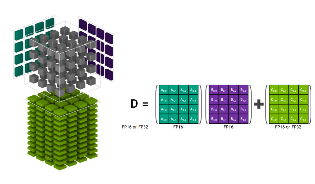
This design is a direct hardware implementation of the principles we've discussed. By performing a dense block of computation (a 4x4 matrix multiply involves 64 multiplications and additions), the Tensor Core achieves an extremely high arithmetic intensity, maximizing the use of its dedicated circuits.

To solidify this concept, let's turn to a couple of resources.

Now, let's see how the video you watched earlier connects the concept of low-precision data types directly to the hardware that leverages them.

The Synergy of Mixed Precision and Tensor Cores

So, why is this combination so powerful? It's not just about using FP16. Naively training a model entirely in FP16 often fails because the limited range and precision cause critical numerical information to be lost. The two most common issues are:

1. Gradient Underflow: Gradients, especially for complex models, can be very small numbers. In FP16, these values might get rounded to zero ("underflow"), effectively stopping the learning process for those weights.
2. Weight Update Issues: Even if the gradient isn't zero, adding a very small gradient update to a larger weight value in FP16 might result in no change at all, as the update is smaller than the representable precision of the weight.

The genius of the Tensor Core's design and the mixed-precision training methodology is how they solve these problems:

• Inputs (A, B): Model weights and activations are cast to FP16. This gives us the memory and bandwidth savings.
• Computation (Multiply): The multiplication of the two FP16 matrices happens at high speed within the Tensor Core.
• Accumulation (Add C): The crucial step is that the resulting products are added to a 32-bit FP32 accumulator (C). By performing the accumulation in high precision, the small updates from the multiplication are not lost to rounding errors. This preserves the integrity of the gradient signal.
• Output (D): The final, high-precision result in D can then be stored back to memory, often being cast back down to FP16 for the next layer's input.

This process allows deep learning workloads to get the best of both worlds: the speed and memory efficiency of 16-bit arithmetic with the numerical stability of 32-bit arithmetic for the most critical step (accumulation).

Architectural and Programming Model Implications

From a computer architecture perspective, this represents a significant shift. Instead of a single thread computing a single element of the output matrix (as with standard CUDA cores), Tensor Core operations are performed at the warp level. An entire warp of 32 threads cooperates to load the matrix fragments into registers, issue the single mma instruction to the Tensor Core, and then store the result. This cooperative model is essential for feeding the specialized hardware efficiently.

Furthermore, to fully leverage Tensor Cores, there are practical constraints. As noted in the NVIDIA documentation, the dimensions of matrices involved in the multiplication (e.g., batch size, feature maps, layer sizes) must typically be multiples of 8. This is a direct consequence of the hardware's fixed-size internal architecture and is a key consideration in model design and data padding for performance optimization.

Conclusion

In this lesson, we've unpacked the role of Tensor Cores, one of the most important architectural innovations for accelerating AI. They are not just "faster cores"; they represent a specialized, co-designed solution that pairs a specific computational pattern (mixed-precision matrix multiplication) with dedicated silicon.

Key Takeaways:

• Mixed precision is the strategic use of lower-precision data types (like FP16) to reduce memory usage and increase bandwidth, combined with higher-precision types (FP32) to maintain numerical accuracy.
• Tensor Cores are specialized hardware units that execute a fused matrix-multiply-accumulate operation (D = A x B + C) at extremely high speed.
• The key to their success is performing the multiplication on low-precision inputs (FP16) but carrying out the accumulation in high precision (FP32), which prevents the loss of small gradient values.
• This approach dramatically increases the effective arithmetic intensity of matrix multiplication, allowing these operations to be strongly compute-bound and fully utilize the GPU's power.
• Using Tensor Cores requires adhering to hardware constraints, such as ensuring matrix dimensions are multiples of 8, a crucial consideration for AI system and model design.

Preview of the Next Module:

This lesson concludes our module on the core execution architecture of the GPU. We've seen how CPUs differ from GPUs, explored the SIMT model, analyzed performance with the Roofline model, and now delved into the specialized Tensor Cores.

Throughout these discussions, a recurring theme has been the critical role of memory. In our next module, GPU Memory Hierarchy and Data Movement, we will systematically explore this topic. Our first lesson will diagram the full GPU memory hierarchy, from the fast, tiny registers on an SM to the large, slower global device memory. Understanding this hierarchy is the next essential step in building your expertise in GPU-accelerated systems.