Distance-Vector vs. Link-State Routing Protocols

Hello! In our last lesson, we mastered the configuration of static and default routes, giving us precise manual control over traffic flow. We acknowledged that while static routes are powerful, they don't scale well in large or changing networks.

This lesson introduces the solution: dynamic routing protocols. These protocols allow routers to automatically learn about remote networks from each other and dynamically adapt to topology changes, such as a link going down. Our goal is to understand the two major families of these protocols: distance-vector and link-state. Differentiating between these two foundational approaches is a critical step toward mastering advanced network routing.

1. The Big Picture: IGP vs. EGP

Before diving into distance-vector and link-state, we need to understand the highest-level classification of routing protocols. This classification is based on the concept of an Autonomous System (AS). An AS is a collection of routers under a single administrative control, like a corporate network or an Internet Service Provider (ISP).

• Interior Gateway Protocols (IGPs): These protocols are used to exchange routing information within a single AS. Their primary goal is fast convergence and optimal path selection within the internal network. RIP, EIGRP, and OSPF are all IGPs. Our focus today is on the different types of IGPs.
• Exterior Gateway Protocols (EGPs): These protocols are used to exchange routing information between different ASes. The internet itself is a massive collection of interconnected ASes. The primary EGP is the Border Gateway Protocol (BGP), which is designed for scalability and policy control over performance.

To get a clear picture of this crucial distinction, please watch the following video segment.

2. Distance-Vector Protocols: Routing by Rumor

The first major family of IGPs is distance-vector. The name itself provides a clue to how it works: routers learn about networks based on distance (a metric, like hop count) and vector (a direction, the next-hop router).

The core behavior of a distance-vector protocol is often described as "routing by rumor." A router running a distance-vector protocol doesn't have a complete map of the network. Instead, it learns about remote networks only from the routing tables of its directly connected neighbors.

Imagine a series of signposts on a highway. Each signpost only tells you the distance to the next town and which road to take to get there; it doesn't show you the entire map of the country.

Key Characteristics:

• View of the Network: Limited to the perspective of its neighbors.
• Updates: Routers typically send their entire routing table to their neighbors at regular intervals (e.g., every 30 seconds for RIP).
• Convergence: Generally slower. If a link fails, the "bad news" has to propagate hop-by-hop through the network, which can sometimes lead to routing loops.
• Resource Usage: Less CPU and memory intensive, making them suitable for simpler or older hardware.
• Examples: Routing Information Protocol (RIP), Interior Gateway Routing Protocol (IGRP).

3. Link-State Protocols: Building a Complete Map

The second family of IGPs, link-state, takes a completely different approach. Instead of relying on neighbors' routing tables, each router builds its own complete map of the network topology.

Here's how it works:

1. Each router sends out Link-State Advertisements (LSAs) that describe itself, its connected links (or "link-states"), and its neighbors.
2. These LSAs are "flooded" throughout the network, so every router receives the LSAs from every other router.
3. Each router assembles all these LSAs into a Link-State Database (LSDB), which is essentially a detailed map of the entire network.
4. With a complete map, each router independently runs the Shortest Path First (SPF) algorithm (specifically, Dijkstra's algorithm) to calculate the best, loop-free path to every destination from its own perspective.

Key Characteristics:

• View of the Network: Each router has a complete, synchronized map of the entire topology.
• Updates: Updates are small, triggered by an event (like a link failing), and contain only the information about the change. They are sent only when needed, not periodically.
• Convergence: Much faster. Because every router has a full map, it can immediately calculate a new best path when it learns of a failure.
• Resource Usage: Requires more CPU and memory to maintain the database and run the SPF algorithm.
• Examples: Open Shortest Path First (OSPF), Intermediate System to Intermediate System (IS-IS).

The following video and reading provide a great direct comparison of these two behaviors.

For a textual summary and to solidify these concepts, you can review the following article.

4. Comparison Summary

The fundamental difference lies in how routers "see" the network. Distance-vector routers see the network through their neighbors' eyes, while link-state routers build their own comprehensive map.

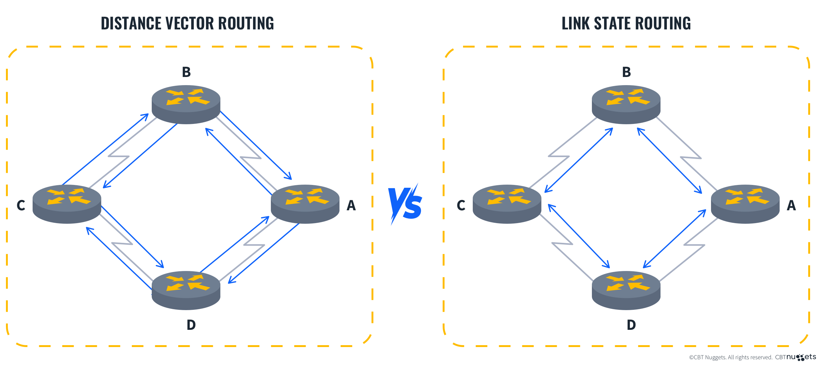
The following chart provides an excellent side-by-side comparison of their key attributes.

A Note on EIGRP: You may have noticed Cisco's EIGRP protocol in the lists. It's often called an advanced distance-vector or hybrid protocol. While it fundamentally operates like a distance-vector protocol (it exchanges routes with neighbors), it incorporates many features of link-state protocols, such as triggered updates, building a topology table, and very fast convergence. For CCNA purposes, it's best to classify it as an advanced distance-vector protocol.

Conclusion

In this lesson, you have learned to distinguish between the two fundamental families of interior routing protocols. This theoretical understanding is crucial for selecting, configuring, and troubleshooting the right protocol for a given network scenario.

Key Takeaways:

• Dynamic routing protocols are categorized into IGPs (within an AS) and EGPs (between ASes).
• Distance-vector protocols work by "routing by rumor," where routers share their routing tables with neighbors. They are simpler but converge more slowly.
• Link-state protocols work by having every router build a complete map of the network. They are more complex and resource-intensive but converge much faster.
• The key differences lie in their network view (partial vs. complete), update mechanism (periodic full tables vs. triggered partial updates), and convergence speed (slow vs. fast).

Now that we have this foundational knowledge, we are ready to dive deep into a specific protocol. In our next lesson, we will begin exploring OSPF, the most widely used link-state protocol in modern enterprise networks. We'll start by examining its core processes for discovering neighbors and building its network map.