IP Reputation System Design

Hello! Welcome back to our course on architecting security products.

In our last lesson, we designed a comprehensive data collection pipeline to gather security signals related to IP addresses from threat intelligence feeds, honeypots, and our own application logs. We now have streams of high-value data flowing into a central point, ready for processing.

This brings us to the core of our IP reputation system. Now that we have the data, how do we transform it into an actionable security signal? This lesson directly addresses that question, focusing on the learning outcome: Design a scoring model and low-latency, real-time lookup architecture for an IP reputation system.

We'll tackle this in two parts:

1. The Scoring Model: We will design a mathematical model to convert raw event data into a quantitative reputation score. This gets to the "first principles" of what reputation means.
2. The Lookup Architecture: We will architect a high-performance, distributed system to serve these reputation scores in real-time with single-digit millisecond latency, a classic system design challenge.

1. Designing the Reputation Scoring Model

At its heart, a reputation score is a numerical representation of trust. An IP address that has recently been observed performing malicious actions should have a "bad" score, while an IP with no negative history should have a "good" or "neutral" score. Our scoring model needs to formalize this logic.

We won't reinvent the wheel. A well-regarded model for this is PRESTA (Spatio-Temporal Reputation Analysis). It's powerful because it elegantly combines two key dimensions:

• Temporal: Events that happened recently are more important than old ones.
• Spatial: The reputation of an IP is influenced by the reputation of its "neighbors" (its subnet and its Autonomous System or AS).

Deconstructing the PRESTA Model

As the paper describes, the raw reputation score for an entity $\alpha$ (like an IP address) within a group $G$ (like a subnet) is calculated by summing up the decayed weights of its historical malicious activity.

The formula is:

Let's break this down from a system design perspective:

• hist(α, G, H): This function returns the history of malicious events for the group. This is precisely what our data collection pipeline from the previous lesson provides! The function would query our analytics database (e.g., Elasticsearch) for all events associated with the IPs in a given group.
• decay(tout, h): This function applies a time penalty. An event's negative impact fades over time. A common choice is an exponential decay function, decay(t) = 2^(-Δt/h), where Δt is the time elapsed since the event and h is the "half-life" of a bad reputation. A longer half-life means an IP stays "bad" for longer.
• size(α, G, tin): This function returns the size of the group. This is the normalization factor. A single bad IP in a huge group (like a large AS) has less impact on the group's overall reputation than a bad IP in a small group (like the IP itself, where size=1).

To get a complete reputation profile for an IP, we would calculate this raw_rep score at multiple spatial granularities and combine them.

So, for any given IP address, our system would compute three primary scores:

1. IP-level Reputation: size() is 1. This captures the specific history of that single IP.
2. Subnet-level Reputation: size() is ~768 (for three /24 blocks). This captures "neighborhood" effects. If an IP is clean but its neighbors are all spamming, it's suspicious.
3. AS-level Reputation: size() is the number of IPs in the Autonomous System. This identifies entire networks that are poorly managed or malicious.

These three scores (rep_ip, rep_subnet, rep_as) can then be fed as features into a simpler model (like a weighted sum or a small machine learning classifier) to produce a final, single reputation score for the IP.

2. Low-Latency, Real-Time Lookup Architecture

Calculating the full PRESTA score can be computationally intensive, as it involves historical lookups. Doing this synchronously for every incoming request to your WAF would add unacceptable latency. The key architectural principle here is to separate the complex, offline scoring from the simple, online lookup.

Let's explore some general principles for low-latency system design before we build our specific architecture.

With these principles in mind, we'll design a multi-tiered lookup architecture. This pattern is common in real-world, high-stakes systems like ad-tech fraud detection.

Tier 1: The Hot Path (Known Bad IPs)

The goal here is to answer "Is this IP known to be bad?" in under 2 milliseconds. We only care about high-confidence, definitively bad IPs in this tier.

Architecture:

1. Bloom Filter: This is a probabilistic data structure that is extremely fast and memory-efficient for set membership tests. We'll keep a Bloom filter in the memory of every lookup service instance. It will be populated with all IPs that currently have a "bad" reputation score.

   • Lookup: Is IP 1.2.3.4 in the bad set? -> Check Bloom filter (~0.1ms).
   • If the filter returns false, we know for certain the IP is not in our high-confidence bad list. We can immediately return a "neutral" score.
   • If the filter returns true, the IP might be in the set (there's a small chance of a false positive). We proceed to the next step.

   
   This diagram shows a hardware-level IP lookup scheme, but the concept is identical for our software architecture: an on-chip (in-memory) Bloom filter acts as a fast, initial check to determine if a more expensive off-chip (Redis) lookup is necessary.

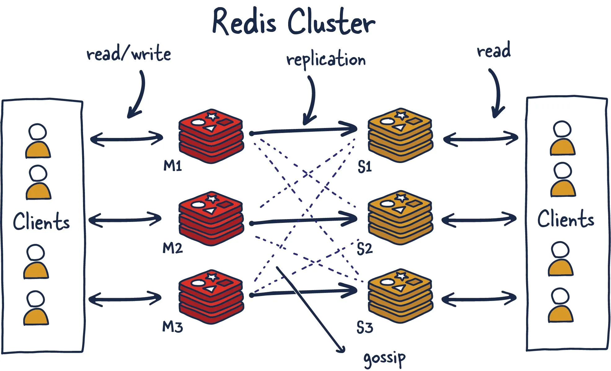
2. In-Memory Key-Value Store (Redis): This is our definitive source of truth for the hot path. We use a distributed Redis cluster for high availability and read scalability.

   • Lookup: If the Bloom filter returned true, we query Redis: GET 1.2.3.4.
   • If Redis returns a score, we return that value. This is a true positive. (1-2ms latency).
   • If Redis returns nil, it was a Bloom filter false positive. We can pass the request to the next tier or return "neutral".

Tier 2: The Warm Path (On-Demand Scoring)

What about IPs that aren't on our "known bad" list but might still be risky? This is where we can use our PRESTA model, but with optimizations.

Architecture:

• As suggested in the PRESTA paper's "Calculation Optimizations" (section 5.6), we can pre-calculate and cache the reputations for entire subnets and ASes offline.
• When an IP is not found in the hot path, the lookup service can:
  1. Fetch the pre-calculated rep_subnet and rep_as scores from a Redis cache.
  2. Perform a quick query against a database (like DynamoDB or Cassandra) for any malicious events from just that single IP in the last few hours. This is a much faster query than a full history scan.
  3. Combine these three components in real-time to generate a moderately accurate, on-demand score.
• This adds more latency (perhaps 10-20ms) but provides a more nuanced score than the simple "bad/not-bad" of the hot path. This is a critical trade-off: higher accuracy for higher latency.

The Offline Scoring Pipeline (The Engine Room)

This is the background process that powers the online lookup tiers. It runs asynchronously and is not in the critical path of user requests.

1. Data Ingestion: A stream processing job (e.g., using Spark, Flink, or a custom service) continuously consumes the normalized security events from the Kafka topic we designed in the last lesson.
2. Scoring: Periodically (e.g., every 5-15 minutes), this job runs the full PRESTA model against the recent historical data stored in our analytics database (Elasticsearch). It calculates rep_ip, rep_subnet, and rep_as for all relevant entities.
3. Tier Updates:
   • It identifies all IPs with a final score above a "high-confidence bad" threshold.
   • It generates a new Bloom filter based on this list of bad IPs.
   • It pushes the full scores for these bad IPs into the Redis hot cache.
   • It pushes the updated rep_subnet and rep_as scores to the Redis warm cache.
   • Finally, it distributes the new Bloom filter file to all running instances of the lookup service, which hot-swap it into memory.

This complete separation ensures that the complex, database-intensive scoring work never impacts the performance of the real-time lookup service.

Conclusion

In this lesson, we designed the brain and the fast-twitch nervous system of our IP reputation product. We moved from raw data to a sophisticated, actionable security score, served at scale with extremely low latency.

Key Takeaways:

• Scoring Model: A robust reputation model like PRESTA considers both temporal decay (recent events matter more) and spatial aggregation (an IP's neighborhood matters).
• Low-Latency Architecture: The key is a multi-tiered approach that separates offline computation from online lookups.
• The Hot Path: For the fastest lookups on known bad IPs, use an in-memory Bloom filter + Redis pattern to achieve sub-2ms latency.
• The Offline Pipeline: A background job must continuously process new data, recalculate scores, and refresh the caches and filters used by the online system. This decoupling is essential for performance and scalability.

Preview of the Next Lesson:

An IP address provides a powerful reputation signal, but sophisticated attackers know how to rotate through thousands of IPs to evade detection. To track the actor, not just the address, we need another layer of identification. In our next lesson, we will "Design passive device fingerprinting techniques using TLS and HTTP header analysis," giving us a way to recognize a specific client or botnet even as it hops across the internet.