Decomposing Price Effects: Substitution and Income

Introduction

Welcome back! In our last lesson, we successfully determined how a rational consumer finds their optimal bundle of goods at the point of tangency between their budget constraint and highest attainable indifference curve. This gave us a static snapshot of consumer choice.

Today, we'll make our model dynamic by asking a crucial question: What happens to this optimal choice when the price of a good changes? You already know from the law of demand that when a price falls, the quantity demanded usually rises. Our goal in this lesson is to look under the hood and understand why this happens. We will decompose the effect of a price change on quantity demanded into a substitution effect and an income effect.

This is a more theoretical, but powerful, part of consumer theory. By breaking down a consumer's response into these two components, we can gain a much deeper understanding of the nature of different goods and the logic behind the demand curve.

Let's begin by reviewing the core ideas.

1. The Total Effect of a Price Change

When the price of a good changes, two things happen simultaneously:

1. The relative prices of the goods change. The good whose price fell is now relatively cheaper.
2. The consumer's real income, or purchasing power, changes. A lower price means your money can now buy more, making you effectively richer.

The consumer's reaction to both of these changes, all at once, is called the total effect.

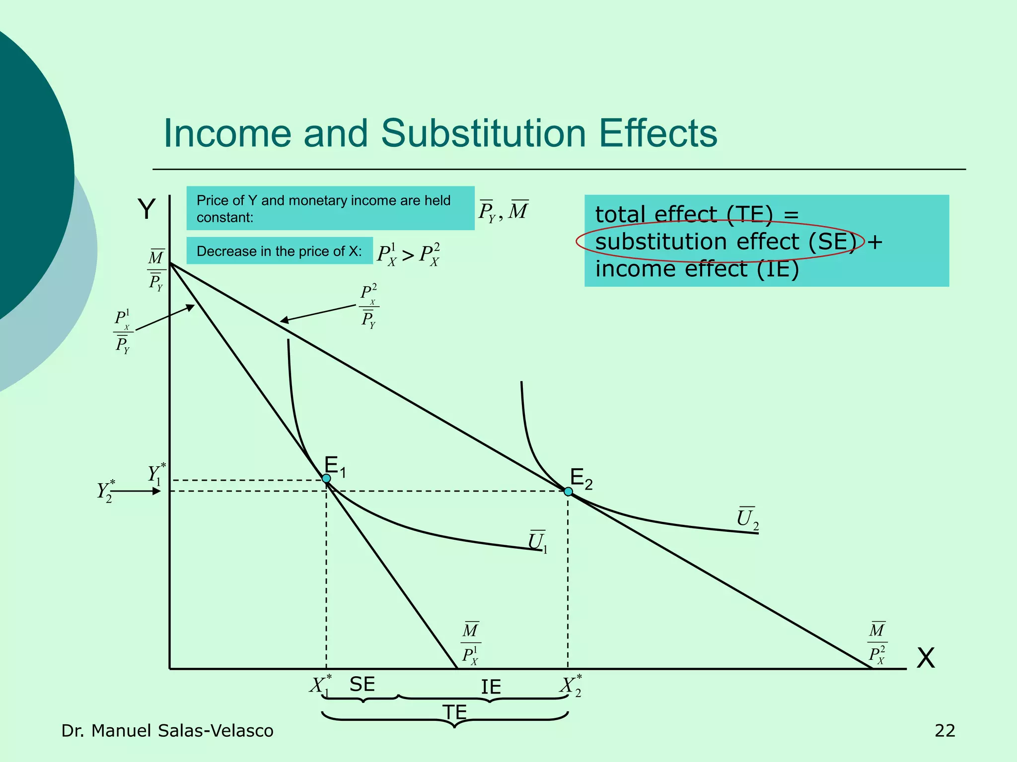
Graphically, a decrease in the price of Good X causes the budget line to pivot outwards. The consumer moves from their initial optimal bundle (Point A) to a new optimal bundle (Point C) on a higher indifference curve. The change in the quantity of Good X from A to C is the total effect.

Our task is to untangle the two forces driving this total effect.

2. Decomposing the Total Effect: Substitution and Income

To isolate the two effects, economists use a clever thought experiment. We break the movement from the initial point (A) to the final point (C) into two steps.

1. The Substitution Effect (SE): This is the change in consumption due solely to the change in relative prices. We isolate it by imagining the consumer's response to the new, cheaper price of Good X if their utility were held constant. In other words, how would they substitute toward the cheaper good along their original indifference curve? This is a movement from the initial point A to a hypothetical intermediate point B.

2. The Income Effect (IE): This is the change in consumption due solely to the change in purchasing power. It's the rest of the change. Having been made "richer" by the price drop, how does the consumer adjust their purchases? This is the movement from the intermediate point B to the final point C, which involves moving to a higher indifference curve.

Therefore, the main relationship is:
Total Effect = Substitution Effect + Income Effect

The following short video provides a clear, animated walkthrough of this decomposition process. It shows exactly how economists construct the hypothetical budget line needed to find the intermediate point and separate the two effects.

To reinforce this graphical method, please read the following text, which walks through the same logic with a static diagram.

3. Direction of Effects and Types of Goods

The real power of this decomposition comes when we consider that the two effects don't always work in the same direction.

The Substitution Effect

The substitution effect is unambiguous: you always substitute towards the good that has become relatively cheaper.

• If price falls, you consume more of it (SE is positive).
• If price rises, you consume less of it (SE is negative).
  There are no exceptions to this rule. It follows directly from the convexity of indifference curves.

The Income Effect

The income effect's direction depends on the type of good:

• Normal Good: When real income rises (due to a price drop), you consume more. The income effect reinforces the substitution effect.
• Inferior Good: When real income rises, you consume less. The income effect works in the opposite direction to the substitution effect.

The following video with MIT's Prof. Jonathan Gruber provides an excellent explanation of how these effects play out for different types of goods. He analyzes a price increase, which is a valuable complementary perspective.

Giffen Goods: The Exception to the Rule

This brings us to a famous, though rare, possibility. What if a good is so strongly inferior that the income effect not only opposes but also overwhelms the substitution effect?

• Price Falls: You are effectively richer. You want to buy so much less of this inferior good (income effect) that it outweighs your desire to substitute towards it because it's cheaper (substitution effect). The net result: a price drop causes you to buy less.
• Price Rises: You are effectively poorer. You want to buy so much more of this inferior good (income effect) that it outweighs your desire to substitute away from it. The net result: a price rise causes you to buy more.

This is called a Giffen good, and it has an upward-sloping demand curve, violating the law of demand. The classic (though debated) example is a staple food like potatoes during a famine. If the price of potatoes rises, a poor family is made so much poorer that they can no longer afford any "better" food (like meat) and must spend all their remaining money on the only thing they can still afford: more potatoes.

Prof. Gruber concludes his segment with a discussion of Giffen goods.

4. A Note on Methods: Hicks vs. Slutsky

The graphical method we have used is known as the Hicksian decomposition, named after Nobel laureate Sir John Hicks. Its defining feature is that it isolates the substitution effect by holding utility constant (staying on the original indifference curve).

There is a related method called the Slutsky decomposition. It isolates the substitution effect by holding purchasing power constant, meaning the consumer is given just enough income to be able to afford their original bundle at the new prices.

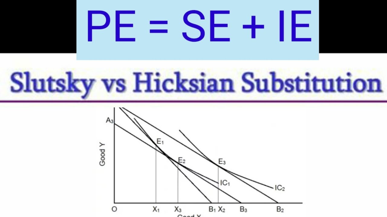
For most applications and for small price changes, the two methods give very similar results. The Hicksian approach is often favored in theoretical economics because holding utility constant is key for welfare analysis. Your analytical background might appreciate that these graphical concepts can be formalized into the Slutsky Equation, a central equation in microeconomic theory, but for this course, the graphical intuition is the most important takeaway.

Conclusion

Today, we took a deep dive into the consumer's response to a price change. Instead of just observing the final result, we developed a powerful theoretical tool to separate the two underlying motivations.

Here are the key takeaways:

• The total effect of a price change on quantity demanded can be decomposed into a substitution effect and an income effect.
• The substitution effect is due to the change in relative prices and always works in the opposite direction of the price change (e.g., a price drop increases quantity via substitution).
• The income effect is due to the change in real purchasing power. For a normal good, it reinforces the substitution effect. For an inferior good, it opposes it.
• This decomposition explains why the law of demand is so robust for normal goods and why, in the rare case of a Giffen good (a highly inferior good), it can be violated.

We now have a complete theoretical foundation for understanding how an individual's consumption choices respond to price changes. In our next lesson, we will put this knowledge to direct use to formally derive an individual's demand curve from the utility-maximization framework we've built over the last several lessons.