Deriving Demand from Utility Maximization

Introduction

Hello! Welcome back. In our last lesson, we deconstructed a consumer's response to a price change into the substitution and income effects. This provided the "why" behind the shift in consumption. Today, we'll put all the pieces together to achieve one of the central goals of consumer theory: we will formally derive an individual's demand curve from the utility-maximization framework.

We will see how a consumer's optimal choices at different price points trace out their personal demand curve. This process connects the abstract model of indifference curves and budget constraints directly to the demand curve we first introduced in Module 2.

By the end of this lesson, you will be able to demonstrate how the familiar downward-sloping demand curve is not just an assumption, but a logical consequence of rational consumer choice. We will approach this both graphically, for intuition, and analytically, to leverage your quantitative background.

1. From Optimal Choice to a Demand Curve: The Graphical Method

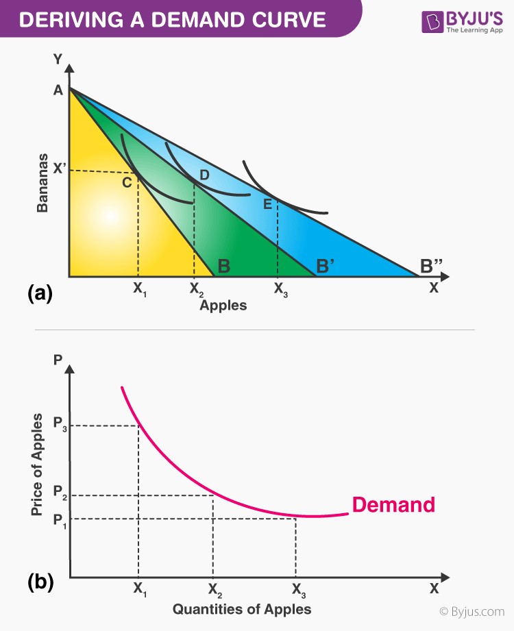
Let's begin with the graphical derivation. The core idea is to observe how the consumer's optimal bundle changes as we vary the price of one good, while holding their income and the price of the other good constant.

The process is straightforward:

1. Find the initial utility-maximizing bundle (tangency point) at the starting price.
2. Decrease the price of one good. This pivots the budget constraint outwards.
3. Find the new utility-maximizing bundle at the new, lower price.
4. Repeat this for several different prices.
5. Plot each price and its corresponding optimal quantity on a separate graph.

The line that connects all the utility-maximizing bundles in the indifference curve diagram is called the price-consumption curve (PCC). The points from the PCC, when plotted in a price-quantity space, form the individual demand curve.

The image below illustrates this two-step process perfectly.

To see this process in motion, let's watch a video that walks through the derivation step-by-step.

Now, let's solidify this with a second example that includes specific numbers, showing how the price is determined from the budget constraint.

2. Linking the Demand Curve's Slope to Income and Substitution Effects

In the last lesson, we saw that the total effect of a price change is the sum of the substitution effect (SE) and the income effect (IE). This decomposition is what determines the slope of the demand curve.

• Normal Goods: When the price of a normal good falls, the SE leads you to buy more (it's relatively cheaper), and the IE also leads you to buy more (your purchasing power has increased). Since both effects push in the same direction, the quantity demanded unambiguously increases. This guarantees a downward-sloping demand curve.

• Inferior Goods: When the price of an inferior good falls, the SE still leads you to buy more. However, the IE now pushes you to buy less (as you become effectively richer, you buy less of the inferior good). As long as the SE is stronger than the IE, the total effect is still an increase in quantity demanded, and the demand curve still slopes downward. This is the case for most inferior goods.

• Giffen Goods (The Rare Exception): A Giffen good is a special type of inferior good where the income effect is so strong that it outweighs the substitution effect. When its price falls, the IE causes such a large decrease in consumption that it overcomes the SE's push for an increase. The net result is that a fall in price leads to a fall in quantity demanded. This results in an upward-sloping demand curve, a violation of the Law of Demand.

The following resource provides a concise summary of these ideas.

3. The Analytical Derivation of Demand

Given your background in technology and analysis, you'll appreciate that we can derive demand functions not just graphically, but also with mathematical optimization. The goal is to solve the consumer's problem to find an equation that gives the optimal quantity of a good, $q_x$, as a function of its price ($P_x$), the price of other goods ($P_y$), and income ($I$). This is the demand function: $q_x=f(P_x,P_y,I)$.

The problem is:
Maximize Utility $U(q_x,q_y)$
Subject to the budget constraint $P_x{q}_x+P_y{q}_y=I$

A powerful technique for solving such constrained optimization problems is the Method of Lagrange Multipliers. You may have encountered this in calculus or other quantitative fields. It allows us to combine the objective function and the constraint into a single equation (the Lagrangian) and solve for the optimal quantities.

The following reading selection provides a formal mathematical treatment. Don't worry about memorizing every step, but focus on understanding the process: setting up the Lagrangian, taking partial derivatives, and solving the resulting system of equations to find the demand functions.

This mathematical derivation confirms what our graphical intuition shows: the optimal quantity a consumer chooses is a function of prices and income. By holding income and other prices constant, we get the relationship between price and quantity demanded—the demand curve itself.

Conclusion

In this lesson, we bridged the gap between the abstract theory of consumer choice and the practical concept of a demand curve. We have now seen from multiple angles—graphical, conceptual, and mathematical—that the demand curve is a direct result of consumers maximizing their utility subject to a budget constraint.

Here are the key takeaways:

• An individual's demand curve is derived by finding their utility-maximizing bundle at various price points and plotting these price-quantity combinations.
• Graphically, the price-consumption curve (PCC) tracks the optimal bundles, which are then used to plot the demand curve.
• The downward slope of the demand curve is explained by the interplay of the substitution and income effects. For normal and most inferior goods, the total effect of a price drop is an increase in quantity demanded.
• Analytically, we can solve the consumer's constrained optimization problem to derive a formal demand function, which gives the optimal quantity for any set of prices and income.

This lesson completes our deep dive into the theory of the consumer. You now have a solid foundation for understanding individual and market demand. In the next module, we will turn our attention to the other side of the market: the producers. We'll begin by exploring the costs of production, laying the groundwork for building a theory of supply.