Optimal Consumer Choice: Tangency Condition

Introduction

Hello! Welcome back to our study of consumer choice. In our last two lessons, we built the essential components of our model. First, we defined the budget constraint, which represents what a consumer can afford based on their income and market prices. Then, we explored the consumer's preferences using an indifference map, which shows what a consumer wants.

Today, we will bring these two concepts together. The goal of this lesson is to answer the central question of consumer theory: How does a rational consumer choose the best possible combination of goods they can afford? This directly addresses the learning outcome: Determine the optimal consumer choice using the tangency condition between the budget constraint and an indifference curve.

We will cover:

• How to find the optimal bundle graphically by superimposing the indifference map onto the budget constraint.
• The economic intuition behind the optimal choice.
• The mathematical condition for optimality, known as the tangency condition.
• A practical example of how to calculate the optimal quantities of two goods.

By the end of this lesson, you will be able to pinpoint the single bundle of goods that maximizes a consumer's satisfaction, laying the groundwork for analyzing how this choice changes when prices or income fluctuate.

1. Finding the Optimal Choice: The Graphical Approach

The consumer's goal is straightforward: to reach the highest possible indifference curve (maximum utility) without going beyond their budget constraint (what's affordable).

Let's visualize this. Imagine placing the consumer's indifference map over their budget constraint.

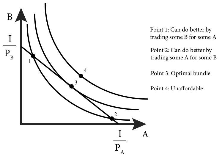
Look closely at the graph:

• Points 1 and 2 are affordable, but they are not optimal. Why? Because the consumer can move to a higher indifference curve (and thus gain more satisfaction) while still staying within their budget.
• Point 4 is on a very high indifference curve, making it highly desirable. However, it lies outside the budget constraint, so it is unaffordable.
• Point 3 is the sweet spot. It is the single point where the budget constraint just touches the highest possible indifference curve. At this point of tangency, the consumer has maximized their utility given their budget. Any other affordable point lies on a lower indifference curve.

The following video provides an excellent animated explanation of this process, bringing the budget line and indifference curves together to find the utility-maximizing bundle.

2. The Tangency Condition: The Mathematics of Optimality

The graphical solution gives us the intuition, but your analytical background will appreciate the precise mathematical condition that defines this optimal point.

At the point of tangency (like Point 3 in the image above), the slope of the budget constraint is exactly equal to the slope of the indifference curve.

Let's recall what these slopes represent from our previous lessons:

1. Slope of the Budget Constraint: This is the ratio of the prices of the two goods, $-P_1/P_2$. It represents the rate at which the market allows the consumer to trade good 2 for good 1.
2. Slope of the Indifference Curve: This is the Marginal Rate of Substitution (MRS). It represents the rate at which the consumer is willing to trade good 2 for good 1 while keeping their utility constant.

Therefore, at the optimal point, the following tangency condition must hold:

(We drop the negative signs as both slopes are negative).

Since we also know that $\text{MRS}=M{U}_1/M{U}_2$, we can write the condition as:

Rearranging this gives us a very intuitive result:

This equation is the heart of consumer choice theory. It says that at the optimal bundle, the marginal utility per dollar spent on good 1 must be equal to the marginal utility per dollar spent on good 2. This is often called the "equal bang for your buck" rule. If it weren't true—say, if $M{U}_1/P_1>M{U}_2/P_2$, the consumer could increase their total utility by spending one less dollar on good 2 and one more dollar on good 1. They would continue this reallocation until the "bang for the buck" is equalized across both goods.

The following reading provides a concise summary of this condition from an intuitive, visual, and mathematical perspective.

3. A Quantitative Example

Let's make this concrete. Given your background as an IT analyst, you'll likely find a step-by-step problem-solving approach helpful. We can find the optimal quantities of goods by solving a system of two equations with two unknowns (the quantity of each good):

1. The Tangency Condition: $\frac{M{U}_1}{M{U}_2}=\frac{P_1}{P_2}$
2. The Budget Constraint: $P_1{X}_1+P_2{X}_2=\text{Income}$

The process involves using the tangency condition to express one good in terms of the other, and then substituting that relationship into the budget constraint to solve for the quantities.

The video below works through a full example, starting from a given utility function and budget.

4. When the Tangency Condition Doesn't Apply: Corner Solutions

The tangency condition works beautifully for "well-behaved" preferences, where the consumer buys a positive amount of both goods (an interior solution). However, in some cases, the optimal choice might be to spend all the budget on just one good. This is called a corner solution.

This often happens with goods that are perfect substitutes. For example, if you see two brands of bottled water as identical and one is cheaper, you will buy only the cheaper one. In this case, your highest indifference curve will hit the corner of your budget set, not be tangent to it.

The reading from EconGraphs that you looked at earlier also discusses these exceptions. For a deeper understanding, you can now read the second half of that article under the heading "When does the tangency condition find the optimal bundle?". It explains why corner solutions occur and mentions other special cases.

Conclusion

In this lesson, we unified the concepts of budget constraints and consumer preferences to find the utility-maximizing choice. This is a cornerstone of microeconomic analysis.

Here are the key takeaways:

• A consumer's optimal choice is the bundle of goods that lies on their budget line and touches the highest possible indifference curve.
• Graphically, this is found at the point of tangency between the budget line and an indifference curve.
• Mathematically, this tangency is expressed by the condition $\text{MRS}=P_1/P_2$, which means the consumer's personal trade-off rate equals the market's trade-off rate.
• This condition can be rearranged into the "equal bang for your buck" rule: $M{U}_1/P_1=M{U}_2/P_2$. The utility gained from the last dollar spent on each good is equal.
• This framework allows us to solve for the exact optimal quantities of goods a consumer will purchase.

We have now established a complete model of how a consumer makes a choice under static conditions. But what happens when those conditions change? In our next lesson, we will use this framework to explore how a consumer's optimal choice changes when the price of a good falls, and we will decompose that change into the income and substitution effects.