Modeling Externalities and Market Inefficiency

Introduction

Welcome back! In our last lesson, we defined externalities as the "spillover" costs or benefits that affect third parties not directly involved in a market transaction. We distinguished between negative externalities, where social costs exceed private costs (like pollution), and positive externalities, where social benefits exceed private benefits (like vaccinations). We concluded that because free markets fail to account for these external effects, they tend to overproduce goods with negative externalities and underproduce goods with positive externalities.

Today, we will build directly on that foundation. Your learning outcome for this lesson is to use a supply-and-demand diagram to show how externalities lead to market inefficiency. We will move from the conceptual to the graphical, translating these ideas into the familiar supply and demand framework. This will allow us to visualize precisely why the market equilibrium is inefficient and to identify the resulting deadweight loss—a quantitative measure of the value lost to society.

Analyzing Negative Externalities Graphically

Let's start with negative externalities, where an activity imposes costs on others. As we discussed, these can arise from production (a factory polluting a river) or consumption (second-hand smoke). The key is that the full cost to society is not captured by the market supply curve.

1. Negative Production Externalities

When a firm's production process creates external costs, its private supply curve does not reflect the true cost to society.

• The supply curve represents the firm's Marginal Private Cost (MPC).
• The Marginal Social Cost (MSC) includes both the private cost and the external cost: $MSC=MPC+\text{Marginal External Cost}$.
• Because the external cost is positive, the MSC curve lies above the MPC (supply) curve.

To see how this creates inefficiency, let's watch a detailed walkthrough.

As the video explained, the market reaches equilibrium at quantity $Q_1$, where the private costs and benefits are equal (MPC = MPB). However, the socially optimal quantity is $Q^{\ast }$, where the social costs and benefits are equal (MSC = MSB).

The key takeaway is that the market leads to overproduction ($Q_1>Q^{\ast }$). For every unit produced between $Q^{\ast }$ and $Q_1$, the marginal social cost of producing it is greater than the marginal social benefit of consuming it. This difference represents a net loss to society, which cumulatively creates the deadweight loss (the shaded triangle).

2. Negative Consumption Externalities

The logic is similar for externalities caused by consumption, but the effect is on the demand side of the market.

• The demand curve represents the consumer's Marginal Private Benefit (MPB).
• The Marginal Social Benefit (MSB) is the private benefit minus the external cost imposed on others: $MSB=MPB-\text{Marginal External Cost}$.
• Because of the external cost, the MSB curve lies below the MPB (demand) curve.

Let's see the graphical representation.

Here again, the market settles at $Q_1$ (where MPB = MPC), but the social optimum is at the lower quantity $Q^{\ast }$ (where MSB = MPC). The market results in overconsumption. The deadweight loss triangle represents the societal welfare lost from consuming units whose social benefit is less than their social cost.

A Deeper Look at Surplus and Inefficiency

To solidify your understanding, let's analyze the inefficiency by explicitly looking at the changes in social surplus. This approach, which is similar to how you might break down a problem in an analytical field, quantifies the inefficiency.

This reading reinforces the central idea: the unregulated market equilibrium maximizes private surplus (for buyers and sellers) but fails to maximize social surplus (for society as a whole). This failure is the essence of the market inefficiency caused by externalities. The quantity that maximizes social surplus is where Marginal Social Benefit = Marginal Social Cost.

Analyzing Positive Externalities Graphically

Now, let's apply the same logic to positive externalities, where an activity confers benefits on others. Here, the market failure is one of underproduction or underconsumption.

1. Positive Consumption Externalities

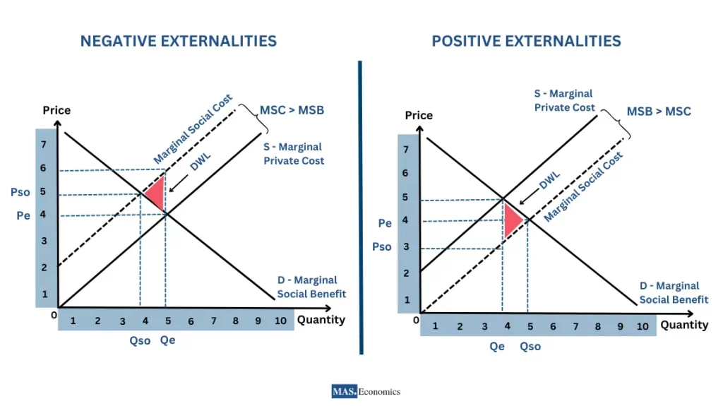
With a positive consumption externality (e.g., higher education, vaccinations), the benefit to society is greater than the benefit to the individual consumer.

• The Marginal Social Benefit (MSB) is greater than the Marginal Private Benefit (MPB): $MSB=MPB+\text{Marginal External Benefit}$.
• The MSB curve lies above the MPB (demand) curve.

The market produces at $Q_{market}$, where the demand curve (MPB) intersects the supply curve (MPC). However, the socially optimal quantity, $Q_{optimal}$, is where the MSB curve intersects the MPC curve.

Since MSB > MPB, it follows that $Q_{market}<Q_{optimal}$. The market produces too little. The deadweight loss is the triangular area representing the net social benefits that could have been gained by producing the additional units from $Q_{market}$ up to $Q_{optimal}$.

2. Positive Production Externalities

While less common, positive production externalities exist (e.g., a beekeeper whose bees pollinate nearby farms). Here, the production process itself generates an external benefit, making the social cost of production lower than the private cost.

• The Marginal Social Cost (MSC) is less than the Marginal Private Cost (MPC): $MSC=MPC-\text{Marginal External Benefit}$.
• The MSC curve lies below the MPC (supply) curve.

The market produces where MPC = MPB, but the social optimum is at a higher quantity where MSC = MPB. Once again, the market leads to underproduction, creating a deadweight loss.

A Framework for Drawing All Four Externality Graphs

You've now seen all four scenarios. To help you master these diagrams, here is a video that provides three simple rules for getting them right every time. This systematic approach should resonate with the logical problem-solving you're familiar with from your IT background.

Let's summarize those invaluable rules:

1. Which Curve Splits?

   • Production externality = Two Cost curves (MSC and MPC).
   • Consumption externality = Two Benefit curves (MSB and MPB).

2. Too Much or Too Little?

   • Negative externality = Market produces too much ($Q_{market}>Q_{optimal}$).
   • Positive externality = Market produces too little ($Q_{market}<Q_{optimal}$).

3. Where is the Deadweight Loss?

   • The deadweight loss triangle always points toward the socially optimal quantity ($Q_{optimal}$). It represents the inefficiency of being at the market quantity.

Conclusion

In this lesson, we used the supply and demand model to graphically demonstrate how externalities lead to market failure. By distinguishing between private and social costs and benefits, we were able to pinpoint the source of inefficiency and measure it as a deadweight loss.

Key Takeaways:

• Negative externalities lead to overproduction because producers or consumers do not face the full social cost of their actions. The market quantity is greater than the socially optimal quantity.
• Positive externalities lead to underproduction because producers or consumers do not capture the full social benefit of their actions. The market quantity is less than the socially optimal quantity.
• In all cases, the divergence between the market equilibrium and the social optimum creates a deadweight loss, which represents a loss of total welfare to society.
• The socially optimal level of output is always found where Marginal Social Cost (MSC) equals Marginal Social Benefit (MSB).

We have now successfully diagnosed the problem. The next logical question is: what can be done about it? In our next lesson, we will explore the solutions, focusing on how government policies like Pigouvian taxes and subsidies can be used to "internalize" the externality, correcting the market failure and guiding the economy toward a more efficient outcome.