Expected Value and Variance: Definitions and Calculations

Hello! Welcome to the next lesson in our journey through probability theory.

In our previous lessons, we built a comprehensive toolkit for describing probability distributions using Probability Mass Functions (PMFs), Probability Density Functions (PDFs), and the unifying Cumulative Distribution Function (CDF). We now know how to represent the full behavior of a random variable. Today, we'll shift our focus from describing the entire distribution to summarizing it with a few key numbers. This lesson is dedicated to the learning outcome: Compute the expected value and variance of a random variable from its definition.

We will explore the two most important summary statistics:

• Expected Value: A measure of the distribution's center, often called the mean.
• Variance: A measure of the distribution's spread or dispersion around its mean.

As someone who has worked with data using Python libraries like Pandas and NumPy, you've likely calculated the mean and variance of datasets. Today, we'll delve into the formal theory behind these concepts, grounding them in the language of probability distributions that we have been developing.

1. Expected Value: The Center of Mass

The expected value of a random variable, denoted as $E[X]$ or ${\mu }_X$, is the long-run average value of the variable if we were to repeat the experiment an infinite number of times. It represents the "center of mass" of the probability distribution.

Discrete Random Variables

For a discrete random variable $X$ that can take on values $x_1,x_2,\dots$ with corresponding probabilities $p_X(x_1),p_X(x_2),\dots$, the expected value is a weighted average of these values, where the weights are the probabilities.

Definition: The expected value of a discrete random variable $X$ is:
$E[X]={\sum }_{x}x\cdot p_X(x)$
where the sum is over all possible values of $X$.

Continuous Random Variables

For a continuous random variable, the concept is analogous. We replace the sum with an integral and the PMF with the PDF.

Definition: The expected value of a continuous random variable $X$ with PDF $f_X(x)$ is:
$E[X]={\int }_{-\infty }^{\infty }x\cdot f_X(x)dx$

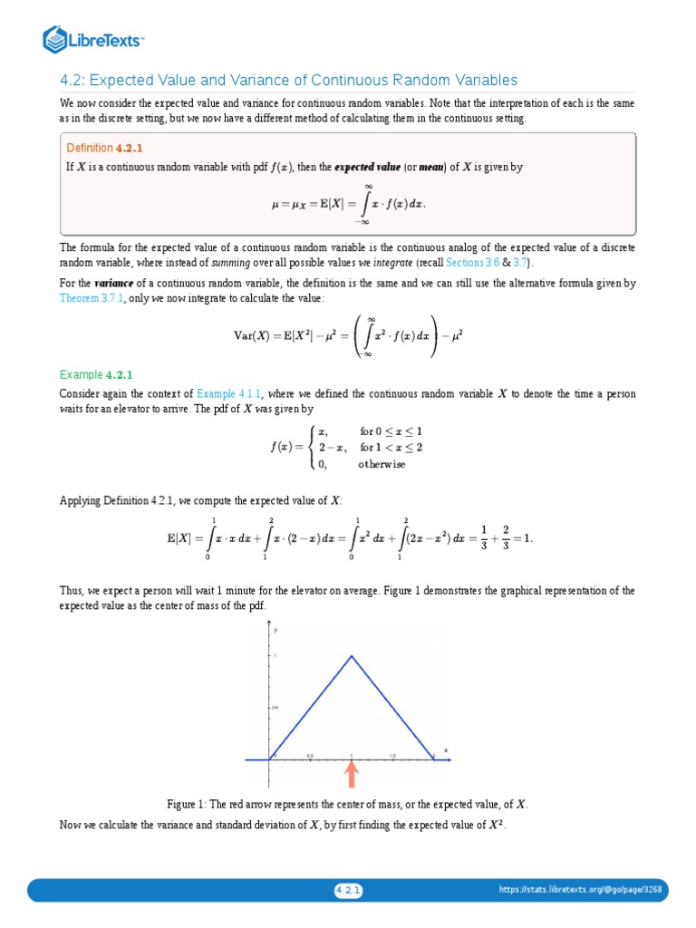
The following reading provides the formal definitions for both cases.

Now, let's watch a worked example of computing the expected value for a continuous random variable from its PDF. Your calculus background will be helpful here.

2. Expectation of a Function and Linearity

Often, we are interested in the expected value of a function of a random variable, say $g(X)$. For example, if $X$ is the daily return of a stock, $g(X)=X^2$ might be part of a risk calculation.

The expected value of $g(X)$ is computed by weighting $g(x)$ by the probability of $X$ being at $x$.

• Discrete: $E[g(X)]={\sum }_{x}g(x)\cdot p_X(x)$
• Continuous: $E[g(X)]={\int }_{-\infty }^{\infty }g(x)\cdot f_X(x)dx$

A critically important property derived from this is the linearity of expectation. For any random variable $X$ and constants $a$ and $b$, it holds that:
$E[aX+b]=aE[X]+b$

This property is fundamental and simplifies many derivations in probability and statistics. Given your preference for mathematical rigor, working through its proof is a valuable exercise.

3. Variance: The Measure of Spread

While the expected value tells us about the center of a distribution, it doesn't describe its spread. Two distributions can have the same mean but vastly different shapes. The variance, denoted $\text{Var}(X)$ or ${\sigma }_X^2$, measures the expected squared deviation from the mean.

Definition: Let $\mu =E[X]$. The variance of $X$ is:
$\text{Var}(X)=E[(X-\mu {)}^2]$

A large variance indicates that the values of $X$ are often far from the mean, while a small variance means they are clustered tightly around it. The standard deviation, ${\sigma }_X=\sqrt{\text{Var}(X)}$, is the square root of the variance and is often used because it has the same units as $X$.

The Computational Shortcut for Variance

Calculating variance directly from the definition can be tedious. A more convenient formula is derived by expanding the definition. This is a classic proof that you should know.

Theorem: $\text{Var}(X)=E[X^2]-(E[X]{)}^2$

Proof:
Let $\mu =E[X]$.
\begin{align*} \text{Var}(X) &= E[(X - \mu)^2] \ &= E[X^2 - 2\mu X + \mu^2] \quad \text{(expanding the square)} \ &= E[X^2] - E[2\mu X] + E[\mu^2] \quad \text{(by linearity of expectation)} \ &= E[X^2] - 2\mu E[X] + \mu^2 \quad \text{(since $2\mu$ and ${\mu }^2$ are constants)} \ &= E[X^2] - 2\mu(\mu) + \mu^2 \quad \text{(since $E[X]=\mu$)} \ &= E[X^2] - 2\mu^2 + \mu^2 \ &= E[X^2] - \mu^2 \ &= E[X^2] - (E[X])^2 \end{align*}

This shortcut is almost always used in practice. To compute the variance, you calculate the expected value of $X$ and the expected value of $X^2$, then combine them.

Let's see this shortcut in action by continuing the previous video example.

Properties of Variance

Just like expectation, variance has a key property related to linear transformations. For constants $a$ and $b$:
$\text{Var}(aX+b)=a^2\text{Var}(X)$

Notice two things:

1. Adding a constant $b$ shifts the entire distribution but doesn't change its spread, so $b$ has no effect on the variance.
2. Multiplying by a constant $a$ scales the deviations. Since variance is based on squared deviations, the scaling factor becomes $a^2$.

The proof is a direct application of the definitions and is an excellent exercise. You can find a clear walkthrough of this proof in the "STAT 24400 Lecture 8" notes on slide 25 (LINK).

Conclusion

In this lesson, we established the formal definitions of expected value and variance, which are fundamental for summarizing probability distributions. You now have the theoretical tools to compute these quantities for any given discrete or continuous random variable.

Key Takeaways:

• Expected Value ($E[X]$) is the probability-weighted average of a random variable's possible values.
  • Discrete: $E[X]=\sum x\cdot p_X(x)$
  • Continuous: $E[X]=\int x\cdot f_X(x)dx$
• Variance ($\text{Var}(X)$) is the expected squared deviation from the mean, measuring the spread of the distribution.
• The shortcut formula for variance, $\text{Var}(X)=E[X^2]-(E[X]{)}^2$, is essential for practical computation.
• The properties of linear transformations are crucial: $E[aX+b]=aE[X]+b$ and $\text{Var}(aX+b)=a^2\text{Var}(X)$.

Preview of the Next Lesson:
We have defined the general methods for computing mean and variance. In the next lesson, we will apply these methods to derive these properties for some of the most important probability distributions in machine learning: the Bernoulli and Binomial distributions. This will move us from general theory to the specific properties of named distributions that you will encounter frequently.