Understanding Cumulative Distribution Functions

Hello! Welcome back to our study of probability theory.

In the last lesson, we defined the Probability Density Function (PDF) for continuous random variables. We established that the PDF, $f_X(x)$, is the derivative of another function, the Cumulative Distribution Function (CDF), $F_X(x)$. This was a crucial step, but we left the CDF itself largely unexplored.

Today, we will put the CDF in the spotlight. This lesson fully addresses the learning outcome: Define and compute cumulative distribution functions (CDFs) for both discrete and continuous random variables. We will see that the CDF is a more fundamental and universal tool than either the PMF or the PDF, as it provides a unified way to describe the distribution of any type of random variable.

1. The Universal Definition of a CDF

While PMFs are for discrete variables and PDFs are for continuous ones, the CDF works for everything. This is because it is defined directly in terms of probability, a concept that applies to all random variables.

Definition: The Cumulative Distribution Function (CDF) of a random variable $X$, denoted $F_X(x)$, is defined as the probability that $X$ will take a value less than or equal to $x$.
$F_X(x)=P(X\le x),\text{for all }x\in \mathbb{R}$
This function "accumulates" probability as $x$ increases from $-\infty$ to $+\infty$. The following video introduces this idea and highlights the universal nature of the CDF.

2. Fundamental Properties of a CDF

Because every CDF is defined in terms of a probability measure, all CDFs, regardless of the underlying random variable, share a set of fundamental properties. Your preference for mathematical rigor will be satisfied here, as these properties are essential for formal proofs in probability and statistics.

Any function $F_X(x)$ that is a CDF must satisfy:

1. Limits at Infinity: The CDF must start at 0 and end at 1.
   ${\lim }_{x\to -\infty }{F}_X(x)=0\text{and}{\lim }_{x\to \infty }{F}_X(x)=1$
   This makes intuitive sense: the probability of $X$ being less than or equal to an infinitely small number is 0, and the probability of it being less than or equal to an infinitely large number is 1.

2. Non-decreasing: As $x$ increases, the CDF can only increase or stay the same. It can never decrease.
   If $a<b$, then $F_X(a)\le F_X(b)$.

3. Right-continuous: The function is continuous from the right. At any point $x$, the limit from the right must equal the function's value at that point.
   ${\lim }_{h\to 0^{+}}{F}_X(x+h)=F_X(x)$
   This property handles the "jumps" we see in discrete CDFs. The value at the jump point is the upper value.

The next video provides a clear explanation of these three characteristic properties.

3. CDFs for Continuous Random Variables

As we saw in the previous lesson, the PDF and CDF are intimately linked through calculus. For a continuous random variable $X$ with PDF $f_X(t)$, the CDF is found by integration.

$F_X(x)=P(X\le x)={\int }_{-\infty }^x{f}_X(t)dt$

This means the value of the CDF at a point $x$ is precisely the area under the PDF curve to the left of $x$.

Let's see how to construct a CDF from a PDF with a concrete example.

To deepen your understanding, the following document provides worked examples for several important continuous distributions. Your background in calculus will make the integration straightforward.

4. CDFs for Discrete Random Variables

For a discrete random variable, we don't integrate a PDF. Instead, we sum the probabilities from the PMF, $p_X(k)$, for all possible outcomes less than or equal to $x$.

$F_X(x)=P(X\le x)={\sum }_{k\le x}{p}_X(k)$

This results in a step function (or staircase function). The function is constant between points of probability mass and "jumps" up at each point where there is a non-zero probability. The height of each jump is equal to the probability mass at that point. This is a direct consequence of the right-continuity property we discussed.

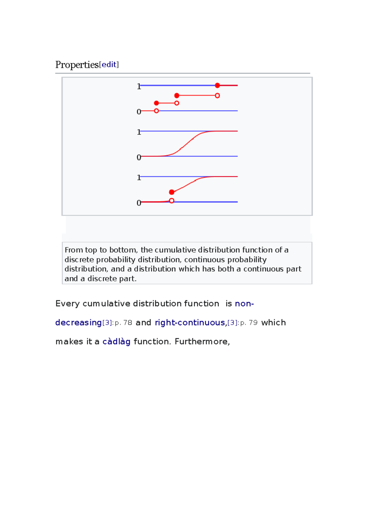
The following video provides an excellent visual walkthrough of constructing a discrete CDF from a given PMF.

You can see the formal mathematical expression for a discrete CDF in the "Lecture 3: Cumulative distribution functions" notes, specifically in the examples for the Bernoulli distribution and a general discrete distribution with finite support (parts 1 and 2 of Example 3.1.2).

Conclusion

In this lesson, we formally defined the Cumulative Distribution Function and established it as a cornerstone of probability theory. It provides a single, unified framework for describing the distribution of any random variable.

Key Takeaways:

• The CDF is universally defined as $F_X(x)=P(X\le x)$.
• All CDFs are non-decreasing, right-continuous, and have limits of 0 at $-\infty$ and 1 at $+\infty$.
• For continuous variables, the CDF is the integral of the PDF, $F_X(x)={\int }_{-\infty }^x{f}_X(t)dt$, resulting in a smooth, continuous function.
• For discrete variables, the CDF is the sum of PMF values, $F_X(x)={\sum }_{k\le x}{p}_X(k)$, resulting in a step function.

Preview of the Next Lesson:
Now that we have a complete set of tools to describe a probability distribution (PMF, PDF, CDF), we can move on to summarizing its key features. In the next lesson, we will explore two of the most important summary statistics: the expected value (a measure of central tendency) and the variance (a measure of spread). We will derive these quantities directly from their definitions using the PMF and PDF.