Bernoulli and Binomial Mean & Variance from PMFs

Hello! Welcome to your next lesson in our study of probability theory.

In the last lesson, we established the formal definitions for two of the most important summary statistics of a random variable: its expected value ($E[X]$) and its variance ($\text{Var}(X)$). We saw that these represent the distribution's center of mass and its spread, respectively. Crucially, we derived the powerful computational formula for variance: $\text{Var}(X)=E[X^2]-(E[X]{)}^2$.

Today, we will apply these tools to two fundamental discrete probability distributions. Your learning outcome for this lesson is to derive the mean and variance of the Bernoulli and Binomial distributions from their Probability Mass Functions (PMFs).

These distributions are not just academic examples; they form the bedrock of modeling binary events, which is central to many machine learning tasks like classification. Given your preference for mathematical rigor, we will derive these properties from first principles.

1. The Bernoulli Distribution

A Bernoulli trial is a single experiment with exactly two possible outcomes: "success" (represented by 1) and "failure" (represented by 0). The Bernoulli distribution models the outcome of such a trial.

Let $X$ be a Bernoulli random variable.

• The parameter is $p$, the probability of success, where $0\le p\le 1$.
• The outcomes are $x\in \{0,1\}$.
• The Probability Mass Function (PMF) is:
  • $P(X=1)=p$
  • $P(X=0)=1-p$

This can be written more compactly as: $P(X=x)=p^x(1-p{)}^{1-x}$ for $x\in \{0,1\}$.

Deriving the Mean and Variance of a Bernoulli Distribution

Let's now derive the mean ($E[X]$) and variance ($\text{Var}(X)$) for a Bernoulli random variable $X\sim \text{Bernoulli}(p)$. The following video provides a clear, step-by-step derivation.

Let's summarize the derivation you just watched.

1. Mean (Expected Value):
We apply the definition of expectation for a discrete random variable, $E[X]={\sum }_{x}x\cdot P(X=x)$.

$$E[X]=(0\cdot P(X=0))+(1\cdot P(X=1))=(0\cdot (1-p))+(1\cdot p)=p$$

So, the mean of a Bernoulli distribution is simply the probability of success, $p$.

2. Variance:
We use the computational shortcut, $\text{Var}(X)=E[X^2]-(E[X]{)}^2$. We already have $E[X]=p$, so we just need $E[X^2]$.

$$E[X^2]=\sum _x{x}^2\cdot P(X=x)=(0^2\cdot (1-p))+(1^2\cdot p)=0+p=p$$

Notice that for a Bernoulli variable, $E[X^2]=E[X]$. This is a unique property because $x^2=x$ for $x\in \{0,1\}$.

Now, we substitute into the variance formula:

$$\text{Var}(X)=E[X^2]-(E[X]{)}^2=p-p^2=p(1-p)$$

So, for $X\sim \text{Bernoulli}(p)$:

• Mean: $E[X]=p$
• Variance: $\text{Var}(X)=p(1-p)$

For a textual reference of this proof, you can consult "Probability Notes with Proofs" (LINK), Chapter 14.

2. The Binomial Distribution

The Binomial distribution describes the number of successes in a fixed number of independent Bernoulli trials.

Let $X$ be a Binomial random variable, $X\sim \text{Binomial}(n,p)$.

• The parameter $n$ is the total number of independent trials.
• The parameter $p$ is the probability of success on each trial.
• The random variable $X$ is the total number of successes, so $X$ can take values $k\in \{0,1,2,\dots ,n\}$.

The PMF is given by the formula:

$$P(X=k)=\left(\genfrac{}{}{0ex}{}{n}{k}\right)p^k(1-p{)}^{n-k}$$

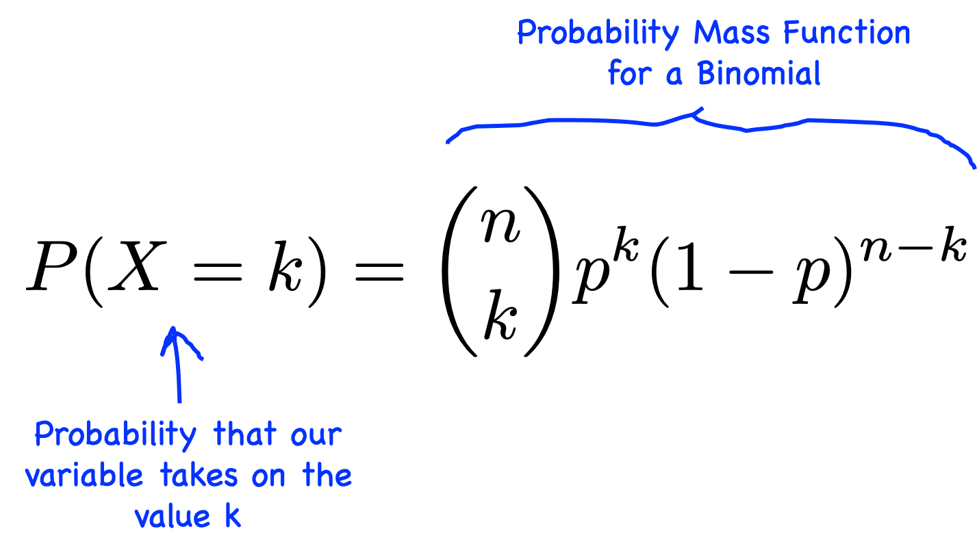
We will derive the mean and variance of the Binomial distribution using two different methods. The first is elegant and relies on the properties of expectation, while the second is a more brute-force algebraic derivation that provides excellent practice with the kind of mathematical manipulation common in machine learning theory.

Method 1: The Sum of Bernoulli Random Variables

The most intuitive way to think about a Binomial random variable $X\sim \text{Binomial}(n,p)$ is as the sum of $n$ independent and identically distributed (i.i.d.) Bernoulli random variables.

Let $Y_1,Y_2,\dots ,Y_n$ be $n$ i.i.d. random variables, where each $Y_i\sim \text{Bernoulli}(p)$. Then $X={\sum }_{i=1}^n{Y}_i$.

This video explains how this insight leads to a very straightforward derivation.

As the video shows, using properties we've learned:

Mean: By the linearity of expectation:

$$E[X]=E\left[\sum _{i=1}^n{Y}_i\right]=\sum _{i=1}^{n}E[Y_i]$$

Since $E[Y_i]=p$ for all $i$, we are just summing $p$ for $n$ times:

$$E[X]=\sum _{i=1}^{n}p=np$$

Variance: Because the trials (the $Y_i$'s) are independent, the variance of the sum is the sum of the variances:

$$\text{Var}(X)=\text{Var}\left(\sum _{i=1}^n{Y}_i\right)=\sum _{i=1}^n\text{Var}(Y_i)$$

Since $\text{Var}(Y_i)=p(1-p)$ for all $i$:

$$\text{Var}(X)=\sum _{i=1}^{n}p(1-p)=np(1-p)$$

This is a powerful and elegant proof that highlights the importance of understanding the relationships between distributions.

Test your understanding!

In your house price prediction project, suppose you are evaluating a new feature. You test it on 10 different data splits. You define "success" as the feature improving your model's accuracy. The probability of success on any given split is 0.6, and the outcomes are independent. Let $X$ be the total number of successful tests. What are $E[X]$ and $\text{Var}(X)$? Explain your reasoning.

Show answer

The random variable $X$ follows a Binomial distribution, $X\sim \text{Binomial}(n=10,p=0.6)$, because it counts the number of successes in a fixed number of independent trials.

Using the formulas derived from the sum of Bernoulli variables:

• Mean: $E[X]=np=10\times 0.6=6$. We expect the feature to improve accuracy on 6 out of the 10 splits.
• Variance: $\text{Var}(X)=np(1-p)=10\times 0.6\times (1-0.6)=10\times 0.6\times 0.4=2.4$.

Method 2: Direct Derivation from the PMF

Now, we will perform the derivation from first principles, using only the PMF. This is more algebraically intensive but is a fantastic exercise. The key challenge lies in manipulating sums involving binomial coefficients.

To prepare for this, let's first review some essential mathematical tools.

With that identity in hand, you are now equipped to follow the full derivation. The following resources walk through the proofs for both the mean and the variance. I recommend watching the video for a dynamic explanation and using the article as a detailed reference to ensure you can follow every step.

Let's recap the key steps in the direct proof for the mean, as this is a classic example of this type of derivation:

1. Start with the definition: $E[X]={\sum }_{k=0}^{n}k\cdot \left(\genfrac{}{}{0ex}{}{n}{k}\right)p^k(1-p{)}^{n-k}$.
2. Simplify the sum: The $k=0$ term is zero, so the sum can start from $k=1$.
3. Apply the key identity: Replace $k\left(\genfrac{}{}{0ex}{}{n}{k}\right)$ with $n\left(\genfrac{}{}{0ex}{}{n-1}{k-1}\right)$.
4. Factor out constants: Pull $n$ and one $p$ out of the sum to get $np\sum \dots$.
5. Change of variables: Let $j=k-1$ and $m=n-1$. This makes the expression inside the sum look familiar.
6. Recognize the sum: The summation becomes ${\sum }_{j=0}^m\left(\genfrac{}{}{0ex}{}{m}{j}\right)p^j(1-p{)}^{m-j}$. This is the sum of all probabilities for a $\text{Binomial}(m,p)$ distribution, which equals 1.
7. Final result: $E[X]=np\cdot 1=np$.

The proof for variance follows a similar pattern but requires the clever step of first computing $E[X(X-1)]$ to simplify the factorial algebra. Mastering these two proofs will significantly strengthen your mathematical toolkit.

Conclusion

In this lesson, you applied the fundamental definitions of mean and variance to derive these properties for two essential discrete distributions.

Key Takeaways:

• For a Bernoulli random variable $X\sim \text{Bernoulli}(p)$:
  • Mean: $E[X]=p$
  • Variance: $\text{Var}(X)=p(1-p)$
• For a Binomial random variable $X\sim \text{Binomial}(n,p)$:
  • Mean: $E[X]=np$
  • Variance: $\text{Var}(X)=np(1-p)$
• There are often multiple valid paths to a proof. The elegant method (using sums of i.i.d. variables) provides deep intuition, while the direct algebraic method builds crucial mathematical skills.

Preview of the Next Lesson:
Having mastered these discrete distributions, we will turn our attention to the most important continuous distribution in all of statistics and machine learning: the Gaussian (or Normal) distribution. In the next lesson, you will derive the mean and variance of the univariate Gaussian distribution from its PDF. This will involve similar principles but will require your calculus skills, particularly integration by parts.