GANs as a Minimax Game

Introduction

In our previous lessons on Variational Autoencoders, we explored a powerful method for generative modeling based on probabilistic principles. We learned to map data to a structured latent space and then sample from that space to generate new data, optimizing an explicit objective function called the Evidence Lower Bound (ELBO). This approach, rooted in variational inference, provides an elegant way to approximate an intractable data distribution.

Today, we pivot to a completely different and revolutionary paradigm for generative modeling: Generative Adversarial Networks (GANs). Instead of defining an explicit probability distribution or a direct loss function like reconstruction error, GANs learn to generate data through a competitive, game-theoretic process. This lesson will introduce the core framework of GANs, breaking down the roles of its two key components and formalizing their interaction as a two-player minimax game, a concept central to the original 2014 paper by Goodfellow et al.

The Adversarial Game

At the heart of a GAN are two neural networks locked in a contest:

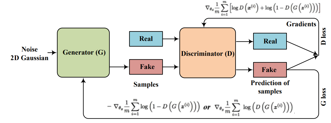
1. The Generator (G): This network's goal is to create synthetic data that is indistinguishable from real data. It takes a random vector from a simple noise distribution (e.g., a Gaussian), denoted $z$, and transforms it into a sample, $G(z)$, that has the same structure as the real data (e.g., an image). The generator is akin to a counterfeiter trying to produce fake currency that looks perfectly genuine.

2. The Discriminator (D): This network's goal is to act as a detective, distinguishing real data from the generator's fakes. It takes a sample, $x$, and outputs a single scalar, $D(x)$, representing the probability that $x$ is a real sample from the training data, not a fake one produced by $G$.

The training process pits these two networks against each other. The discriminator is trained on a mix of real images (from the dataset) and fake images (from the generator). The generator is trained based on the discriminator's feedback: if the discriminator successfully identifies its output as fake, the generator must adjust its parameters to produce more convincing fakes. Over time, this adversarial dynamic drives the generator to produce samples of remarkable fidelity.

The video below offers an excellent intuition for this setup using the counterfeiter-and-police analogy.

Formalizing the Game: The Minimax Objective

To turn this intuitive idea into a trainable system, we need to define a mathematical objective. The entire framework can be expressed as a single value function, $V(D,G)$, which represents the "payoff" in this game. The discriminator tries to maximize this payoff, while the generator tries to minimize it.

Let's derive this from first principles.

The Discriminator's Objective

The discriminator's task is a standard binary classification problem. For any given input $x$, it outputs $D(x)$, the probability that $x$ is real.

• For a real sample $x$ drawn from the true data distribution $p_{data}(x)$, the ideal output is $D(x)=1$.
• For a fake sample $G(z)$, where $z$ is drawn from a noise distribution $p_z(z)$, the ideal output is $D(G(z))=0$. The probability of it being real is zero.

Given this, what loss function would we use to train a binary classifier? As we saw in Module 4, the binary cross-entropy is the natural choice. The discriminator wants to maximize the log-probability of correctly classifying both real and fake samples. This translates to:

1. Maximizing $\log (D(x))$ for real samples.
2. Maximizing $\log (1-D(G(z)))$ for fake samples (since $1-D(G(z))$ is the probability of the sample being fake).

Averaging over all possible real and fake samples, the discriminator's goal is to maximize the following value function:

$$\underset{D}{\max }V(D,G)={\mathbb{E}}_{x\sim p_{data}(x)}[\log D(x)]+{\mathbb{E}}_{z\sim p_z(z)}[\log (1-D(G(z)))]$$

The Generator's Objective

The generator has the opposite goal. It wants to fool the discriminator. A successful generator produces samples $G(z)$ that the discriminator classifies as real, meaning $D(G(z))$ is close to 1. Looking at the value function $V(D,G)$, the generator has no control over the first term, ${\mathbb{E}}_{x\sim p_{data}(x)}[\log D(x)]$, as it doesn't involve $G$. Its sole focus is on the second term.

To fool the discriminator, the generator wants $D(G(z))$ to be high. This is equivalent to making $\log (1-D(G(z)))$ very low (i.e., a large negative number). Therefore, the generator's objective is to minimize the same value function that the discriminator is trying to maximize.

The Minimax Equation

Combining these two opposing goals gives us the central equation of GANs—a minimax game:

$$\underset{G}{\min }\underset{D}{\max }V(D,G)={\mathbb{E}}_{x\sim p_{data}(x)}[\log D(x)]+{\mathbb{E}}_{z\sim p_z(z)}[\log (1-D(G(z)))]$$

This elegant equation captures the entire adversarial process. The generator $G$ tries to minimize the objective, while the discriminator $D$ simultaneously tries to maximize it. This is a zero-sum game where one player's gain is the other's loss.

To see this mathematical formulation developed from the ground up, the following resources are excellent.

The Theoretical Optimum: Reaching Equilibrium

The brilliance of the minimax formulation is not just its elegance, but its theoretical properties. The original paper proved that this game has a unique equilibrium point. Let's think about what happens when the system reaches this equilibrium.

The generator gets so good that its generated distribution, $p_g$, is identical to the real data distribution, $p_{data}$. At this point, the discriminator can no longer tell the difference between real and fake samples. For any input $x$, the sample is equally likely to have come from the real dataset or the generator.

What does this imply for the discriminator's output? If it cannot distinguish the two, its best strategy is to guess. Thus, for any sample $x$, $D(x)=1/2$. The discriminator is completely confused, outputting a 50% probability for every input.

This is the Nash Equilibrium of the game. At this point:

1. The generator's distribution perfectly matches the data distribution: $p_g=p_{data}$.
2. The discriminator outputs $1/2$ everywhere.
3. Neither player can improve its outcome by unilaterally changing its strategy.

The minimax objective, when optimized perfectly, is equivalent to minimizing the Jensen-Shannon Divergence (JSD) between the real data distribution and the generated data distribution. The JSD is a symmetric and smoothed version of the KL divergence we've seen before. It is zero if and only if the two distributions are identical. Therefore, by playing this minimax game, the generator is implicitly driven to make its output distribution match the true data distribution perfectly.

The following resources dive into the mathematical proof that shows the connection between the GAN objective and Jensen-Shannon Divergence, providing the formal justification for why this adversarial game works.

Conclusion

In this lesson, we have laid the foundation for understanding Generative Adversarial Networks. We have moved from the probabilistic approach of VAEs to a game-theoretic framework where two networks, a generator and a discriminator, compete to improve each other.

Key Takeaways:

• GANs consist of two networks: A Generator that creates data from noise, and a Discriminator that classifies data as real or fake.
• Training is an adversarial process: The generator tries to fool the discriminator, and the discriminator tries to get better at catching the generator's fakes. This competition drives the generator to produce highly realistic data.
• The objective is a minimax game: The entire process is captured by a single value function $V(D,G)$ that the discriminator aims to maximize and the generator aims to minimize.
• The theoretical optimum is a Nash Equilibrium: At the point of equilibrium, the generator's output distribution is identical to the real data distribution ($p_g=p_{data}$), and the discriminator is maximally confused ($D(x)=1/2$). This corresponds to minimizing the Jensen-Shannon Divergence between the two distributions.

Preview of the Next Lesson:

While the theory of GANs is elegant, their practical training is notoriously difficult. The beautiful equilibrium we discussed is hard to reach. In the next lesson, we will investigate the common failure modes of GAN training, such as mode collapse (where the generator produces only a limited variety of samples) and training instability (where the generator and discriminator fail to converge). Understanding these challenges is the first step toward exploring the many architectural innovations designed to make GANs more stable and powerful.