The Reparameterization Trick in VAEs

Introduction

In our last lesson, we derived the full objective function for a Variational Autoencoder, the Evidence Lower Bound (ELBO), and decomposed it into two intuitive parts: a reconstruction term and a KL divergence regularizer. We ended with a critical cliffhanger. The reconstruction term, ${\mathbb{E}}_{z\sim q_{\varphi }(z|x)}[\log p_{\theta }(x|z)]$, involves an expectation over the approximate posterior $q_{\varphi }(z|x)$. In practice, we estimate this expectation by sampling a latent vector $z$ from the distribution produced by our encoder.

This presents a fundamental problem for training. The parameters of our encoder, $\varphi$, define the very distribution we are sampling from. The sampling process itself is a stochastic, non-differentiable operation. How can we possibly use backpropagation to compute the gradient of the loss with respect to $\varphi$ if there's a random "gap" in the computational graph?

This lesson introduces the elegant solution to this problem: the reparameterization trick. We will explore precisely why this trick is necessary from a first-principles perspective and then see how it masterfully restructures the network's data flow to enable end-to-end training with gradient descent.

The Problem: Gradients of Expectations

Let's formalize the issue. Our goal is to compute the gradient of the ELBO with respect to the encoder parameters, $\varphi$. The problematic part involves the reconstruction term:

$${\nabla }_{\varphi }{\mathbb{E}}_{z\sim q_{\varphi }(z|x)}[f(z)]$$

where for simplicity, $f(z)=\log p_{\theta }(x|z)$ represents the reconstruction log-likelihood produced by the decoder.

If the expectation was over a distribution that did not depend on $\varphi$, say $p(z)$, we could simply swap the gradient and the expectation:

$${\nabla }_{\varphi }{\mathbb{E}}_{z\sim p(z)}[f_{\varphi }(z)]={\mathbb{E}}_{z\sim p(z)}[{\nabla }_{\varphi }{f}_{\varphi }(z)]$$

This resulting expectation can be easily approximated using Monte Carlo sampling: draw a few samples of $z$ from $p(z)$, compute the gradient ${\nabla }_{\varphi }{f}_{\varphi }(z)$ for each, and average the results. Backpropagation does this automatically.

However, in our case, the distribution $q_{\varphi }(z|x)$ itself depends on $\varphi$. When we expand the definition of the expectation and apply the product rule for derivatives, we get a more complex expression:

$${\nabla }_{\varphi }{\mathbb{E}}_{z\sim q_{\varphi }(z|x)}[f(z)]={\nabla }_{\varphi }\int q_{\varphi }(z|x)f(z)dz=\int {\nabla }_{\varphi }[q_{\varphi }(z|x)f(z)]dz$$ $$=\int ({\nabla }_{\varphi }{q}_{\varphi }(z|x))f(z)dz+\int q_{\varphi }(z|x)({\nabla }_{\varphi }f(z))dz$$

The second term is fine and looks like the expectation of a gradient. But the first term, $\int ({\nabla }_{\varphi }{q}_{\varphi }(z|x))f(z)dz$, is troublesome. It involves the gradient of the probability density function itself, ${\nabla }_{\varphi }{q}_{\varphi }(z|x)$, which we generally don't know how to compute or sample from. This means a naive Monte Carlo estimate of the gradient will be incorrect, as it would ignore this first term completely. This is the core mathematical reason why backpropagation fails here.

The following reading provides a more formal and rigorous explanation of this problem, cutting through the common but imprecise "we can't backpropagate through a random node" justification.

The Solution: Separating Randomness from Parameters

The insight behind the reparameterization trick is to re-express the process of sampling $z$ in a way that isolates the source of randomness.

Imagine you want to draw a number from a Gaussian distribution with a specific mean $\mu$ and standard deviation $\sigma$. One way is to sample directly from $\mathcal{N}(\mu ,{\sigma }^2)$. Another, equivalent way is to:

1. Sample a random number $ϵ$ from a fixed, standard normal distribution, $\mathcal{N}(0,1)$.
2. Scale this number by $\sigma$.
3. Shift it by $\mu$.

The result, $z=\mu +\sigma \cdot ϵ$, is a random variable with the desired distribution $\mathcal{N}(\mu ,{\sigma }^2)$. The key is that the randomness now comes from an external, fixed source ($ϵ$), while $\mu$ and $\sigma$ are deterministic parameters that transform this randomness.

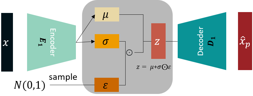
This is precisely the "trick" we apply in a VAE. Instead of having the encoder output a stochastic node $z\sim \mathcal{N}({\mu }_{\varphi }(x),{\Sigma }_{\varphi }(x))$, we have it output the deterministic parameters ${\mu }_{\varphi }(x)$ and ${\sigma }_{\varphi }(x)$. We then sample $ϵ$ from a standard normal distribution $\mathcal{N}(0,I)$ and compute $z$ deterministically.

The video below provides a fantastic, high-level visual explanation of this process.

Applying the Trick to the VAE

Let's see how this transforms our VAE's architecture.

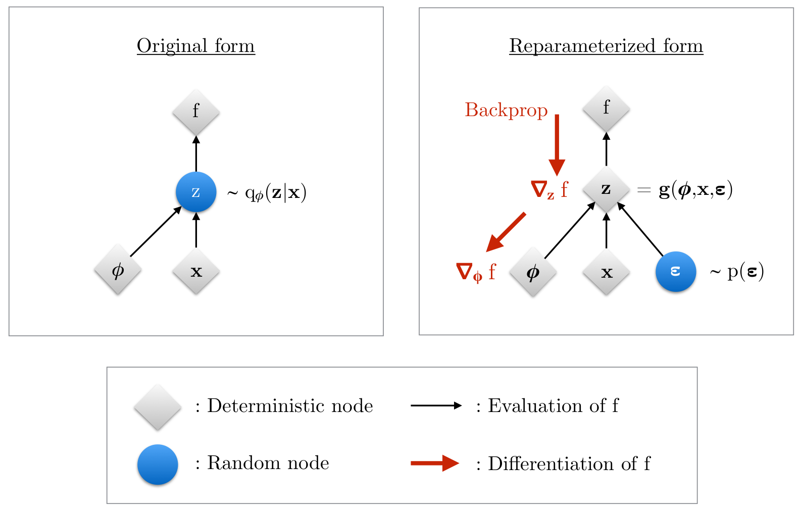
Original (Problematic) Form:

1. Input $x$ goes into the encoder network.
2. The encoder outputs parameters ${\mu }_{\varphi }(x)$ and ${\sigma }_{\varphi }(x)$.
3. A stochastic sampling operation draws $z\sim \mathcal{N}({\mu }_{\varphi }(x),\text{diag}({\sigma }_{\varphi }(x{)}^2))$.
4. $z$ is passed to the decoder.

Reparameterized Form:

1. Input $x$ goes into the encoder network.
2. The encoder outputs deterministic parameters ${\mu }_{\varphi }(x)$ and ${\sigma }_{\varphi }(x)$.
3. A random vector $ϵ\sim \mathcal{N}(0,I)$ is sampled (this is considered an input to the system, not an internal operation).
4. The latent vector $z$ is computed deterministically: $z={\mu }_{\varphi }(x)+{\sigma }_{\varphi }(x)\odot ϵ$, where $\odot$ denotes element-wise multiplication.
5. This deterministic $z$ is passed to the decoder.

Notice the crucial change. The path from the parameters $\varphi$ (which determine $\mu$ and $\sigma$) to the final loss is now composed entirely of deterministic, differentiable operations. The randomness has been "pushed out" to an input node.

The Mathematical Payoff

Now let's revisit our gradient calculation. The reconstruction term was ${\mathbb{E}}_{z\sim q_{\varphi }(z|x)}[f(z)]$. With the trick, we can rewrite $z$ as a function $g(\varphi ,x,ϵ)={\mu }_{\varphi }(x)+{\sigma }_{\varphi }(x)\odot ϵ$. The expectation is no longer over $q_{\varphi }$, but over the fixed distribution of noise, $p(ϵ)=\mathcal{N}(0,I)$.

Our gradient calculation becomes:

$${\nabla }_{\varphi }{\mathbb{E}}_{p(ϵ)}[f(g(\varphi ,x,ϵ))]$$

Since $p(ϵ)$ does not depend on $\varphi$, we can now safely swap the gradient and the expectation:

$$={\mathbb{E}}_{p(ϵ)}[{\nabla }_{\varphi }f(g(\varphi ,x,ϵ))]$$

This expression is exactly what we need! It's an expectation of a gradient. We can get an unbiased estimate of it via Monte Carlo sampling:

1. Sample ${ϵ}^{(l)}$ from $\mathcal{N}(0,I)$.
2. Compute the deterministic value $z^{(l)}={\mu }_{\varphi }(x)+{\sigma }_{\varphi }(x)\odot {ϵ}^{(l)}$.
3. Compute the reconstruction loss and its gradient ${\nabla }_{\varphi }\log p_{\theta }(x|z^{(l)})$ via backpropagation.
4. Average these gradients over a few samples (in practice, often just one sample per data point $x$ is sufficient).

The following resources provide a complete walkthrough, connecting the high-level intuition to the final, trainable loss function.

Conclusion

In this lesson, we tackled the final major hurdle in training a Variational Autoencoder. We moved from an intuitive sense of "not being able to backpropagate through randomness" to a formal understanding of why the gradient of an expectation is problematic when the distribution's parameters are being optimized.

The reparameterization trick provides a mathematically sound and practical solution. By reframing the sampling process to isolate the source of randomness, it creates a fully differentiable path from the encoder's parameters to the final loss, enabling end-to-end training with standard backpropagation.

Key Takeaways:

• The Problem: Training a VAE requires taking the gradient of the ELBO with respect to the encoder parameters $\varphi$. This is problematic because the expectation in the reconstruction term is over a distribution $q_{\varphi }(z|x)$ that itself depends on $\varphi$, which prevents a simple interchange of the gradient and expectation operators.
• The Trick: The reparameterization trick rewrites the sampling of a latent vector $z$ as a deterministic transformation of a fixed noise variable $ϵ$. For a Gaussian VAE, this is $z={\mu }_{\varphi }(x)+{\sigma }_{\varphi }(x)\odot ϵ$, where $ϵ\sim \mathcal{N}(0,I)$.
• The Solution: This moves the stochasticity to an input layer, making the computational path from $\varphi$ to the loss fully differentiable. The gradient of the expectation becomes the expectation of the gradient, which can be estimated via Monte Carlo sampling (i.e., backpropagation).

Preview of the Next Lesson:

Having mastered the architecture and training of VAEs, we have a complete understanding of a powerful generative model. Now, we will turn our attention to a completely different paradigm for generative modeling. In the next lesson, we will introduce Generative Adversarial Networks (GANs), exploring how an adversarial, two-player game between a generator and a discriminator can be used to produce stunningly realistic data.