Understanding GAN Failure Modes

Introduction

In our last lesson, we established the elegant theoretical foundation of Generative Adversarial Networks. We framed the training process as a two-player minimax game between a generator and a discriminator, whose equilibrium point corresponds to the generator's distribution perfectly matching the real data distribution. This equilibrium minimizes the Jensen-Shannon Divergence (JSD) between the two, providing a solid mathematical justification for why GANs should work.

However, theory and practice often diverge. While the concept of a Nash Equilibrium is powerful, achieving it is another matter entirely. This lesson delves into the practical challenges and common failure modes that make training GANs notoriously difficult. We will move from the ideal world of game theory to the complex dynamics of gradient-based optimization, exploring why the adversarial process can become unstable. By understanding these failure modes—specifically training instability, vanishing gradients, and mode collapse—we set the stage for appreciating the architectural and theoretical innovations developed to overcome them.

The Unstable Game: Why Convergence is Not Guaranteed

The minimax objective we derived is not a standard optimization problem. In a typical supervised learning task, you minimize a static loss function. The "topography" of the loss surface doesn't change. In a GAN, you have two agents, the generator $G$ and the discriminator $D$, updating their parameters simultaneously. The update for $G$ changes the loss landscape for $D$, and vice-versa. This dynamic can prevent the system from settling into a stable equilibrium.

Imagine a simple non-cooperative game where one player controls a variable $x$ to minimize the function $f(x,y)=xy$, while another player controls $y$ to minimize $g(x,y)=-xy$.

• The gradient for the first player is $\frac{\partial f}{\partial x}=y$. So, the update rule is $x\leftarrow x-\eta y$.
• The gradient for the second player is $\frac{\partial g}{\partial y}=-x$. So, the update rule is $y\leftarrow y-\eta (-x)=y+\eta x$.

The only equilibrium point is at $(0,0)$. However, if you start anywhere else and apply these updates, the parameters $(x,y)$ will spiral away in ever-increasing orbits rather than converging. GAN training can suffer from a similar, albeit much higher-dimensional, instability.

The following reading provides a great summary of the key problems in GAN training, starting with this difficulty of achieving a Nash equilibrium.

Failure Mode 1: Vanishing Gradients

The reading you just completed introduces two critical ideas: the difficulty of finding a Nash Equilibrium and the concept of distributions on low-dimensional manifolds. Let's connect these to the problem of vanishing gradients.

In our last lesson, we saw that the GAN objective is equivalent to minimizing the JSD. This holds true if the discriminator is optimal. Now, let's consider the practical implications.

Socratic Question: What do you think happens to the generator's learning signal if the discriminator becomes perfect at its job—that is, it can distinguish real from fake samples with 100% accuracy?

...

If the discriminator $D$ is perfect, its output $D(x)$ will be 1 for any real sample and 0 for any generated sample $G(z)$. The generator's loss is a function of $\log (1-D(G(z)))$. As $D(G(z))$ approaches 0, the expression $1-D(G(z))$ approaches 1, and $\log (1)=0$.

The problem isn't just that the loss is low; it's that the gradient of the loss with respect to the generator's parameters vanishes. The discriminator's output function, typically a sigmoid, becomes completely flat in the regions where the generator is producing samples. There is no gradient signal for the generator to follow to improve its outputs. It's like trying to find the bottom of a valley by following the slope, but you're standing on a perfectly flat plateau.

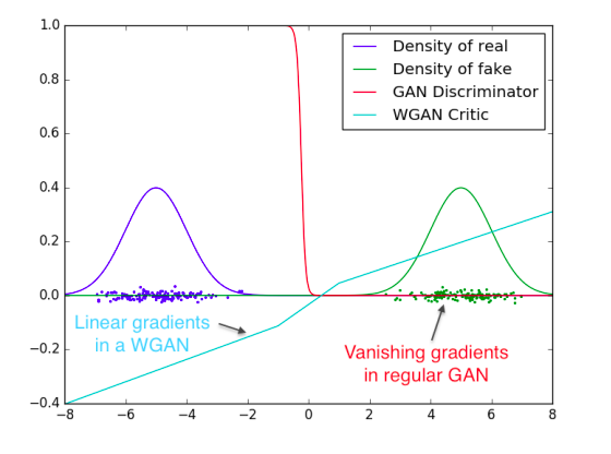
The concept of low-dimensional manifolds from the reading explains why the discriminator can become perfect so easily. Real-world data (like 64x64 images of faces) and the data produced by the generator (mapping from a, say, 100-dimensional latent vector) do not occupy the full 12,288-dimensional pixel space. They lie on much lower-dimensional, complex surfaces. Early in training, it's almost certain that these two manifolds will be disjoint. If they are disjoint, a perfect discriminator that separates them always exists.

This leads to a fundamental dilemma in GAN training:

• If the discriminator is too weak, the generator's loss doesn't accurately approximate the JSD, so the training signal is not meaningful.
• If the discriminator is too strong, its gradients saturate, and the generator receives no training signal at all.

Training a GAN becomes a delicate balancing act.

Failure Mode 2: Mode Collapse

Perhaps the most famous failure mode of GANs is mode collapse. This occurs when the generator learns to produce only a single sample, or a very limited variety of samples, that can fool the discriminator. Instead of capturing the full diversity of the training data, the generator "collapses" onto a few modes of the data distribution.

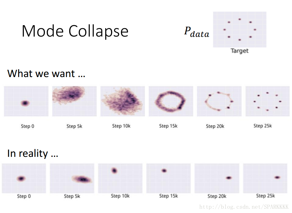
Why does this happen?

The generator's objective at each step is simply to win the current game against the current discriminator. If it discovers a single output that is highly plausible to the discriminator, the path of least resistance for minimizing its loss is to produce that one output repeatedly. The standard GAN objective provides no explicit incentive for the generator to explore and cover all the modes of the data distribution. The adversarial game can fall into a degenerate equilibrium where the generator produces a single realistic sample and the discriminator learns to reject only that specific sample, without pushing the generator to explore other possibilities.

This video segment explains the intuition behind mode collapse.

A Consequence: Meaningless Loss Curves

A final, practical consequence of this instability is that the loss values of the generator and discriminator are often not reliable indicators of training progress or sample quality. Unlike in supervised learning, where a decreasing loss almost always signals a better model, GAN losses can oscillate wildly while image quality improves, or they can converge while the model suffers from mode collapse. This makes hyperparameter tuning and model selection a significant challenge, often relying on manual inspection of generated samples over time.

Conclusion

Today, we've explored the harsh reality behind the elegant theory of GANs. The adversarial dynamic, while powerful, is inherently unstable and prone to failure.

Key Takeaways:

• Training is Unstable: The GAN minimax game does not guarantee convergence. The simultaneous updates by the two players can lead to oscillations or divergence rather than a stable Nash Equilibrium.
• Vanishing Gradients are a Major Obstacle: When the discriminator becomes too effective—which happens easily when the real and generated data distributions lie on disjoint, low-dimensional manifolds—it provides no useful gradient signal to the generator.
• Mode Collapse Limits Diversity: The generator may learn to produce only a limited set of outputs that fool the discriminator, failing to capture the true variety of the data distribution.
• Loss is Not a Reliable Metric: The values of the generator and discriminator loss do not necessarily correlate with the quality or diversity of the generated samples, making training difficult to monitor.

Preview of the Next Lesson:

These problems—instability, vanishing gradients, mode collapse—all stem from a fundamental aspect of the original GAN formulation: the choice of the Jensen-Shannon Divergence as the distance metric to minimize. As we've seen, the JSD saturates when distributions are disjoint, causing these issues.

The next major breakthrough in generative modeling came from recognizing this core problem and proposing a different metric. In our next lesson, we will introduce the Wasserstein GAN (WGAN), which replaces the JSD with the Wasserstein (or "Earth-Mover's") distance. This seemingly simple change leads to a profoundly more stable training process and provides a loss that actually correlates with sample quality, directly addressing the failures we've discussed today.