DDPM: Forward and Reverse Processes

Introduction

In our previous lessons on Generative Adversarial Networks (GANs), we concluded that their training instability often stems from the limitations of the Jensen-Shannon Divergence, especially when the real and generated data distributions are disjoint. This can lead to vanishing gradients and mode collapse, making the adversarial game notoriously difficult to win.

Today, we shift our focus to an entirely different and remarkably successful generative paradigm: Denoising Diffusion Probabilistic Models (DDPMs). Instead of the adversarial dynamics of GANs, diffusion models are inspired by principles from non-equilibrium thermodynamics. They approach the problem of generation not as a single, complex transformation from latent space to data, but as a gradual, multi-step process.

This lesson will introduce the two fundamental components of DDPMs. We will first describe the forward process, a fixed procedure that systematically destroys information in an image by adding Gaussian noise. Then, we will explore the reverse process, which involves training a neural network to methodically undo this noising process, learning to generate data by denoising a pure noise signal. By the end, you will understand the core mechanism that allows these models to generate stunningly high-quality and diverse images.

The Core Idea: Diffusion and Denoising

At its heart, a diffusion model operates on a beautifully simple principle. Imagine you have a clear image, $x_0$.

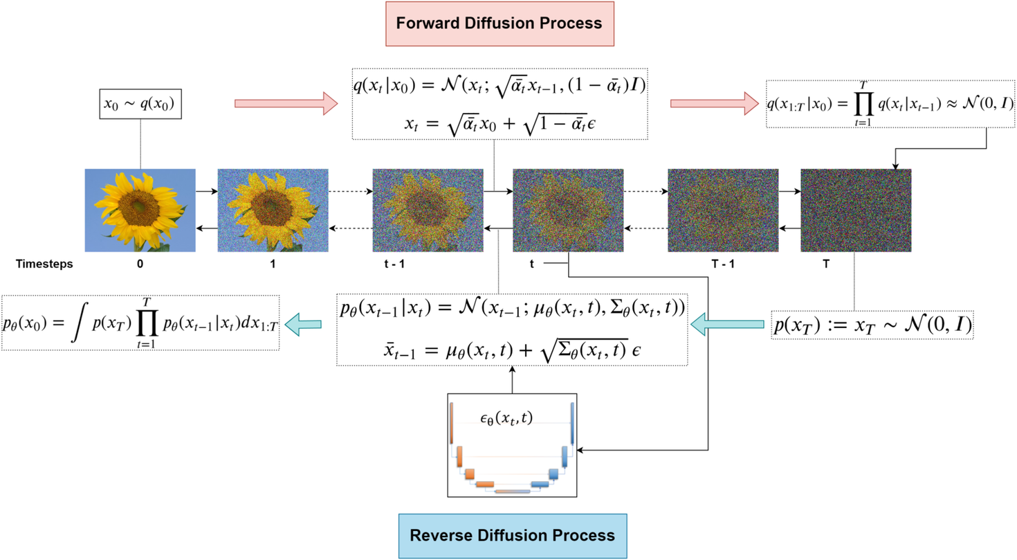
1. Forward (Diffusion) Process: You begin a process of adding a small amount of Gaussian noise to the image. You repeat this over and over again, for a large number of timesteps, $T$. After each step, the image becomes slightly noisier. By the final timestep $T$, the original image is completely overwhelmed by the cumulative noise, and what remains is indistinguishable from a sample drawn from a standard Gaussian distribution. This process is fixed and requires no learning; it's a pre-defined recipe for data destruction.

2. Reverse (Denoising) Process: The generative magic happens here. We now train a neural network to reverse this process. The network's task is, given a noisy image $x_t$ at some timestep $t$, to predict a slightly less noisy image $x_{t-1}$. If this model can learn to perform this single-step denoising operation accurately, we can start with pure noise ($x_T$) and iteratively apply the model $T$ times, gradually removing noise at each step, until a clean, coherent image $x_0$ emerges.

This two-stage mechanism is visualized in the following diagram, which shows an image of a sunflower being progressively noised in the forward process and an architecture for reversing this.

To begin, let's watch a short, high-level overview of this concept.

The Forward Process: A Fixed Markov Chain

Let's formalize the diffusion process. We define it as a Markov chain, which means that the state at any given timestep $t$, denoted as $x_t$, depends only on the state at the immediately preceding timestep, $x_{t-1}$.

At each step, we sample $x_t$ from a Gaussian distribution whose mean is a scaled version of $x_{t-1}$ and whose variance is fixed. The transition is defined as:

$$q(x_t|x_{t-1})=\mathcal{N}(x_t;\sqrt{1-{\beta }_t}{x}_{t-1},{\beta }_t\mathbf{I})$$

Let's break down this equation:

• $\mathcal{N}(x;\mu ,{\sigma }^2\mathbf{I})$ denotes a Gaussian distribution with mean $\mu$ and variance ${\sigma }^2$.
• ${\beta }_t$ is a small, positive constant that defines the variance schedule. It controls how much noise is added at step $t$. These are hyperparameters, typically set to increase from a small value (e.g., $10^{-4}$) to a larger one (e.g., $0.02$) over $T$ steps (e.g., $T=1000$).
• $\sqrt{1-{\beta }_t}{x}_{t-1}$ is the mean of the distribution. We slightly shrink the previous image.
• ${\beta }_t\mathbf{I}$ is the variance. We add Gaussian noise with variance ${\beta }_t$.

We can re-write this process using the reparameterization trick, which makes it clear how a sample $x_t$ is constructed:

$$x_t=\sqrt{1-{\beta }_t}{x}_{t-1}+\sqrt{{\beta }_t}{\mathbf{ϵ}}_{t-1},\text{where }{\mathbf{ϵ}}_{t-1}\sim \mathcal{N}(0,\mathbf{I})$$

The "Shortcut" Property

A key property of this formulation is that we don't need to iteratively apply the noising step $t$ times to find $x_t$. We can derive a closed-form expression to sample $x_t$ directly from the original image $x_0$.

Let ${\alpha }_t=1-{\beta }_t$ and ${\bar{\alpha }}_t={\prod }_{s=1}^t{\alpha }_s$ (the cumulative product of all ${\alpha }_s$). Through recursive substitution, it can be shown that:

$$q(x_t|x_0)=\mathcal{N}(x_t;\sqrt{{\bar{\alpha }}_t}{x}_0,(1-{\bar{\alpha }}_t)\mathbf{I})$$

Or, using the reparameterization trick again:

$$x_t=\sqrt{{\bar{\alpha }}_t}{x}_0+\sqrt{1-{\bar{\alpha }}_t}\mathbf{ϵ},\text{where }\mathbf{ϵ}\sim \mathcal{N}(0,\mathbf{I})$$

This equation is fundamental to the entire DDPM framework. It tells us that any noisy image $x_t$ can be expressed as a simple linear combination of the original image $x_0$ and a single Gaussian noise sample $\mathbf{ϵ}$. This allows us to directly generate training pairs $(x_t,x_0)$ by simply picking a random timestep $t$ and a random noise vector $\mathbf{ϵ}$.

As $t\to T$, the value of ${\bar{\alpha }}_t$ approaches zero. Consequently, the term $\sqrt{{\bar{\alpha }}_t}{x}_0$ vanishes, and $x_T$ is effectively just a sample from $\mathcal{N}(0,\mathbf{I})$, achieving our goal of turning data into pure noise.

To dive deeper into the mathematics of the forward process, the following resources are excellent.

The Reverse Process: Learning to Denoise

Now for the hard part: reversing the diffusion. Our goal is to learn the distribution $p_{\theta }(x_{t-1}|x_t)$, which allows us to take a noisy image $x_t$ and sample a slightly cleaner version $x_{t-1}$.

Socratic Question: Knowing the forward transition $q(x_t|x_{t-1})$, what mathematical tool would you first reach for to try and define the reverse transition $p(x_{t-1}|x_t)$?

...

Your first instinct should be Bayes' theorem:

$$p(x_{t-1}|x_t)=\frac{q(x_t|x_{t-1})p(x_{t-1})}{p(x_t)}$$

However, we immediately hit a wall. Evaluating $p(x_t)=\int q(x_t|x_0)p_{\text{data}}(x_0)d{x}_0$ requires integrating over the entire (unknown) data distribution, making it intractable.

The Trick: Condition on $x_0$

The key insight of diffusion models is that the reverse posterior is tractable if we also condition on the starting image $x_0$: $q(x_{t-1}|x_t,x_0)$. Applying Bayes' theorem here gives:

$$q(x_{t-1}|x_t,x_0)=\frac{q(x_t|x_{t-1},x_0)q(x_{t-1}|x_0)}{q(x_t|x_0)}$$

Because the forward process is Markovian, $q(x_t|x_{t-1},x_0)$ simplifies to $q(x_t|x_{t-1})$. All three terms on the right are known Gaussian distributions we defined in the forward process. A remarkable property of Gaussians is that this combination results in another Gaussian distribution. After some non-trivial algebra (which you can find in the resources), we find that $q(x_{t-1}|x_t,x_0)=\mathcal{N}(x_{t-1};{\tilde{\mu }}_t(x_t,x_0),{\tilde{\beta }}_t\mathbf{I})$, where the mean ${\tilde{\mu }}_t$ is a function of $x_t$ and $x_0$, and the variance ${\tilde{\beta }}_t$ is a function of the $\beta$ schedule.

Parameterizing the Reverse Step

This gives us a target. We know what the reverse step should look like if only we knew the original image $x_0$. Since we don't know $x_0$ during generation (that's what we are trying to create!), we train a neural network $p_{\theta }$ to approximate this posterior.

Given that the true posterior is Gaussian, we parameterize our learned reverse transition $p_{\theta }(x_{t-1}|x_t)$ as a Gaussian as well:

$$p_{\theta }(x_{t-1}|x_t)=\mathcal{N}(x_{t-1};{\mu }_{\theta }(x_t,t),{\Sigma }_{\theta }(x_t,t))$$

The neural network's job is to take a noisy image $x_t$ and the timestep $t$ as input and predict the parameters (mean ${\mu }_{\theta }$ and variance ${\Sigma }_{\theta }$) of the distribution for the previous, cleaner image $x_{t-1}$.

The original DDPM paper simplifies this further by setting the variance to a fixed constant (${\Sigma }_{\theta }(x_t,t)={\sigma }_t^2\mathbf{I}$) and only training the network to predict the mean ${\mu }_{\theta }(x_t,t)$.

The Final Leap: Predicting Noise

The final, crucial design choice is how to parameterize the mean ${\mu }_{\theta }$. We could train the network to predict it directly. However, we can use our shortcut equation $x_t=\sqrt{{\bar{\alpha }}_t}{x}_0+\sqrt{1-{\bar{\alpha }}_t}\mathbf{ϵ}$ to re-express the mean ${\tilde{\mu }}_t(x_t,x_0)$ in terms of $x_t$ and $\mathbf{ϵ}$. This re-parameterization reveals that predicting the mean is mathematically equivalent to predicting the noise $\mathbf{ϵ}$ that was added to create $x_t$.

Empirically, training a network ${\mathbf{ϵ}}_{\theta }(x_t,t)$ to predict the noise component was found to be much more stable and effective. This transforms the complex task of distribution modeling into a straightforward regression problem: given a noisy image $x_t$, predict the noise that it contains.

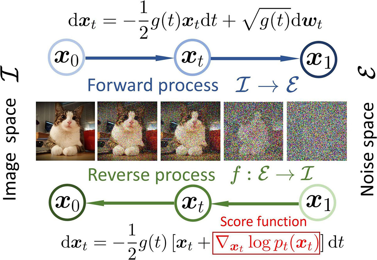
The following video segments provide an excellent walkthrough of these ideas.

Conclusion

In this lesson, we have dissected the core mechanics of Denoising Diffusion Probabilistic Models, establishing the conceptual and mathematical foundation for this powerful class of generative models.

Key Takeaways:

• Two-Process System: DDPMs consist of a fixed forward (diffusion) process that gradually adds Gaussian noise to data, and a learned reverse (denoising) process that iteratively removes it.
• Forward Process is a Fixed Markov Chain: The forward process $q(x_t|x_{t-1})$ is defined by a pre-set variance schedule $\{{\beta }_t\}$. A key property is the "shortcut," which allows sampling a noisy image $x_t$ directly from the original $x_0$ in one step: $x_t=\sqrt{{\bar{\alpha }}_t}{x}_0+\sqrt{1-{\bar{\alpha }}_t}\mathbf{ϵ}$.
• Reverse Process is Learned Denoising: The reverse process aims to learn $p_{\theta }(x_{t-1}|x_t)$. This is framed as approximating the true but intractable posterior $q(x_{t-1}|x_t,x_0)$.
• Noise Prediction is the Objective: The model is parameterized as a Gaussian, and training is simplified to a regression task where a neural network ${\mathbf{ϵ}}_{\theta }(x_t,t)$ learns to predict the noise component of a noisy image $x_t$.

Preview of the Next Lesson:

Now that we understand the what and why of the forward and reverse processes, the next logical step is to understand how we train the model to perform this noise prediction task. In the next lesson, we will derive the simplified DDPM training objective function. We will see how the complex objective of maximizing the data log-likelihood (via the Evidence Lower Bound) elegantly reduces to a simple Mean Squared Error loss between the true noise and the predicted noise.