The Short-Run Phillips Curve: Inflation-Unemployment Trade-off

Introduction

Welcome back! In our previous lesson, we explored how shifts in aggregate demand and supply cause inflation. We saw that demand-pull inflation, driven by an increase in aggregate demand (AD), leads to both a higher price level and higher output. Since higher output generally means lower unemployment, this implies an interesting relationship: a situation with higher inflation might be accompanied by lower unemployment.

Today, we will formalize this observation. Our goal is to explain the short-run Phillips curve and the trade-off between inflation and unemployment. This model provides a different lens through which to view the short-run dynamics of the economy, particularly the choices and constraints faced by policymakers. It builds directly on your understanding of the AD-AS model, showing how the same economic events can be represented in a new framework.

1. The Phillips Curve: A Short-Run Trade-off

In the 1950s, economist A.W. Phillips discovered a stable, inverse relationship between the rate of wage inflation and the unemployment rate in the UK. This finding was later generalized to represent a trade-off between price inflation and unemployment. This relationship became known as the Phillips Curve.

The core idea is that in the short run, an economy faces a trade-off: to achieve lower unemployment, it might have to accept higher inflation, and to achieve lower inflation, it might have to tolerate higher unemployment.

Let's start by reading a brief introduction to the concept.

As the text explains, the Phillips curve is a downward-sloping curve with the inflation rate on the vertical axis and the unemployment rate on the horizontal axis. A point high up on the curve represents a combination of high inflation and low unemployment, while a point lower down represents low inflation and high unemployment.

2. Connecting the Phillips Curve to the AD-AS Model

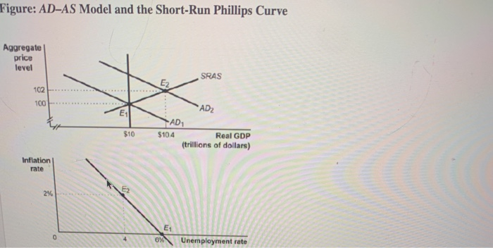
The Phillips curve isn't a separate, independent theory; it's a direct consequence of the short-run aggregate supply (SRAS) curve being upward-sloping. Let's make this connection explicit, as your analytical background will make this dual-model perspective quite powerful.

Recall what happens during demand-pull inflation:

1. Aggregate demand (AD) increases (shifts to the right).
2. The economy moves up along the fixed SRAS curve.
3. The result is a higher price level (inflation ↑) and higher real GDP (output ↑).
4. Since higher output requires more labor, the unemployment rate falls (unemployment ↓).

So, a rightward shift of the AD curve corresponds to a movement up and to the left along the short-run Phillips curve (SRPC).

The following image perfectly illustrates this connection.

Let's watch a video that walks through this linkage for both positive and negative demand shocks.

The key takeaway is that changes in aggregate demand cause a movement along the SRPC. Policymakers who use fiscal or monetary policy to influence AD are, in effect, choosing a point on this short-run trade-off curve.

3. Shifts of the Short-Run Phillips Curve

In the 1970s, many economies, including the U.S., experienced stagflation—simultaneously high inflation and high unemployment. This was a phenomenon the simple Phillips curve couldn't explain, as it suggested we should have one or the other, not both. What happened? The Phillips curve itself had shifted.

The SRPC shifts when the short-run aggregate supply (SRAS) curve shifts. Remember our lesson on cost-push inflation? A negative supply shock (like a surge in oil prices) shifts the SRAS curve to the left. Let's trace the consequences:

1. SRAS shifts left.
2. The economy moves up along the fixed AD curve.
3. The result is a higher price level (inflation ↑) and lower real GDP (output ↓).
4. Since output falls, the unemployment rate rises (unemployment ↑).

This gives us the painful outcome of stagflation. On a Phillips curve diagram, this means that for any given level of unemployment, the inflation rate is now higher. This is represented as a rightward shift of the entire SRPC.

The most important factor that shifts the SRPC is a change in inflationary expectations. If workers and firms expect 3% inflation next year, they will build that into wage negotiations and price-setting. This raises costs and shifts the SRAS curve left, which in turn shifts the SRPC to the right.

The following video provides an excellent summary of what causes movements along the curve versus shifts of the curve.

To summarize the rule:

• Movement along SRPC ⟷ Shift in AD
• Shift of SRPC ⟷ Shift in SRAS (often due to supply shocks or changes in inflation expectations)

4. The Phillips Curve as a Policy Tool

For a time, the Phillips curve was seen as a "policy menu." Governments believed they could choose their preferred combination of inflation and unemployment. Stimulate demand to lower unemployment (at the cost of higher inflation), or dampen demand to lower inflation (at the cost of higher unemployment).

However, the experience of the 1970s showed this was too simplistic. Trying to permanently keep unemployment below its "natural" rate through demand stimulus would lead to accelerating inflation, as expectations would continuously adjust, shifting the SRPC further and further to the right. This led to the distinction between the short-run and long-run Phillips curves. While our focus today is the short-run curve, it's important to know that most economists believe there is no long-run trade-off. In the long run, the economy returns to its natural rate of unemployment regardless of the inflation rate (the vertical line in the image above).

For a bit more context on this historical evolution and its relevance today, please read the following article.

Conclusion

In this lesson, we have connected our understanding of the AD-AS model to the short-run Phillips curve. You can now see how events that shift aggregate demand and supply play out in terms of the relationship between inflation and unemployment.

Key Takeaways:

• The Short-Run Phillips Curve (SRPC) illustrates an inverse relationship between the inflation rate and the unemployment rate.
• This trade-off is a direct reflection of an upward-sloping SRAS curve.
• Shifts in aggregate demand cause movements along the SRPC. An increase in AD leads to higher inflation and lower unemployment.
• Shifts in short-run aggregate supply, often driven by supply shocks or changes in inflation expectations, cause the entire SRPC to shift. A negative supply shock shifts the SRPC to the right, leading to stagflation.

Preview of the Next Lesson:

The short-run Phillips curve highlights the difficult choices policymakers face. If the economy is in a recession (high unemployment, low inflation), they might want to stimulate aggregate demand. The tools to do this fall into two main categories: fiscal policy and monetary policy. In our next module, we will begin our deep dive into Fiscal Policy. Our first lesson will cover the fundamentals: describing the main components of government revenue and expenditure, which are the building blocks of the government's budget.