Batching's Impact on GPU Performance in Training and Inference

Recommended resources

The freely available resources this lesson will direct you to.

Introduction

In our last lesson, we took a deep dive into optimizing a single, critical operation: the attention mechanism. We saw how a hardware-aware algorithm like FlashAttention avoids materializing a large intermediate matrix, transforming a memory-bandwidth-bound operation into a more compute-bound one. This dramatically improved performance by reducing data movement between the GPU's slow HBM and fast on-chip SRAM.

Today, we elevate our perspective from optimizing a single kernel to optimizing the throughput of the entire system. While efficient kernels are crucial, GPUs achieve their peak performance only when they are fed a continuous, substantial stream of parallel work. This lesson addresses the fundamental technique for achieving this: batching.

Our learning outcome is to describe how batching strategies affect GPU utilization and throughput in both training and inference. We will explore the core trade-offs of batching, differentiate its application in the predictable world of training versus the dynamic environment of inference, and analyze the state-of-the-art strategies used to maximize hardware efficiency.

1. The Fundamental Trade-off: Throughput vs. Latency

At its core, batching is about aggregating multiple independent tasks (e.g., processing different data samples or user requests) and executing them together as a single, larger unit of work. This has a direct and significant impact on two key system metrics:

Throughput: The rate at which the system can process work, often measured in samples per second, tokens per second, or requests per second. By providing the GPU with large matrices and tensors, batching increases the arithmetic intensity and allows the hardware's massive parallelism to be fully exploited, thus maximizing throughput.
Latency: The time it takes to process a single task, from start to finish. Batching can increase latency because an individual request might have to wait for a full batch to be assembled before processing can begin.

GPU Batching Trade-offs: Throughput vs. Interactivity — This image illustrates the core trade-off. On the left, batching multiple user requests maximizes GPU utilization and throughput. On the right, processing a single user's request immediately minimizes their individual latency but results in poor GPU utilization and low overall throughput.

This trade-off is central to system design. A system designed for offline data processing (like model training) will be heavily optimized for throughput, while an interactive, real-time application (like a chatbot) must also carefully manage latency to ensure a good user experience.

2. Batching in Model Training

In the context of model training, you are already familiar with batch_size as a key hyperparameter in frameworks like PyTorch or TensorFlow. From a systems perspective, the choice of batch size is a primary lever for controlling training performance.

Larger batch sizes create larger matrix multiplications, which are more efficient for the GPU to process. This improves hardware utilization and increases training throughput (samples/sec). However, simply using the largest batch size that fits in GPU memory is not always the optimal strategy. This is where the statistics of the optimization process intersect with the hardware performance.

Increasing the batch size yields diminishing returns in terms of how much each gradient step reduces the loss. This leads to the concept of a critical batch size.

Critical batch-size in deep learning

The following article provides an excellent theoretical and empirical exploration of the 'critical batch size'. It connects the systems-level goal of maximizing throughput with the machine learning goal of efficient convergence.

Please read the 'Introduction' and 'Gradient descent and optimal learning rate' sections. As you read, focus on: The definition of critical batch size as the point where increasing the batch size no longer yields linear improvements in training speed. The derivation that shows the optimal learning rate (\eta_{\text{opt}}) depends on the batch size (B) and a 'batch-noise' term (\mathcal{B}_{\text{noise}}). The formula \eta_{\text{opt}} = \frac{1 }{1 + \mathcal{B}_{\text{noise}}/B} \eta_{\text{max}} is key.

The core insight from the paper is that there is an optimal batch size that balances two factors:

Computational Efficiency: The time it takes to process one batch. Larger batches are more efficient from a hardware perspective.
Statistical Efficiency: The number of gradient updates (steps) required to reach convergence. Smaller, noisier batches can sometimes explore the loss landscape more effectively.

The critical batch size, $B_{crit}$ , marks the point where the benefit of faster computation from larger batches is outweighed by the reduced statistical efficiency. Training with a batch size much larger than $B_{crit}$ can waste computational resources, as you are taking fewer, more expensive steps that are not proportionally more effective. This is a crucial concept for designing cost-effective large-scale training systems.

3. Batching in Inference: The Challenge of Dynamic Workloads

Inference workloads present a starkly different and more complex challenge than training. While training batches are typically uniform (e.g., all images are 224x224), inference requests are highly dynamic and unpredictable in both input length and required output length.

Consider a large language model (LLM) serving requests:

A short question might have 10 input tokens and require 50 output tokens.
A document summarization task might have 4000 input tokens and require 200 output tokens.

To understand why this is challenging, we must first distinguish the two phases of LLM inference.

Mastering LLM Techniques: Inference Optimization

This NVIDIA developer blog post provides a concise explanation of the two distinct phases of LLM inference, which have very different performance characteristics.

Read the section 'Understanding LLM inference', which covers the 'Prefill phase' and 'Decode phase'. Note the distinction between the highly parallel, compute-bound prefill and the sequential, memory-bound decode.

The prefill phase is computationally intensive but efficient, while the decode phase is a long sequence of small, memory-bound steps. This dynamism and two-phase nature make simple batching strategies ineffective.

Static Batching

The most basic approach is static batching. The system waits to collect a number of requests, pads them all to the length of the longest request in the batch, and processes them together.

The problem is significant inefficiency:

Wasted Compute: A large portion of the GPU's work is spent on processing padding tokens, which contribute nothing to the output.
Idle Time (Head-of-Line Blocking): All requests in the batch must wait for the single longest request to finish generating its output. GPU resources are tied up, and throughput plummets.

Continuous (In-flight) Batching

To solve this, modern inference servers use continuous batching, also known as in-flight batching. This is a far more sophisticated scheduling technique.

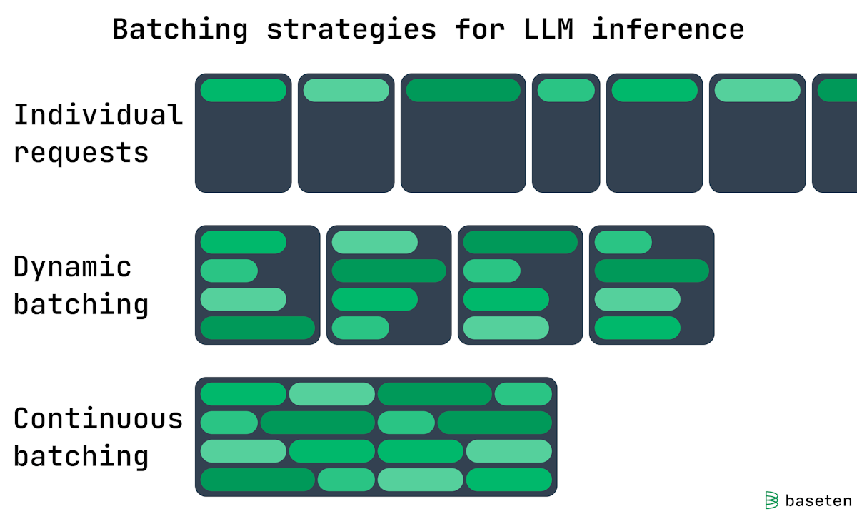
Batching Strategies for LLM Inference — This diagram visually contrasts three batching strategies. 'Individual requests' shows very low utilization. 'Dynamic (Static) batching' improves utilization but leaves idle gaps between batches. 'Continuous batching' shows the highest utilization by dynamically scheduling requests to fill nearly all available processing capacity.

Instead of rigid batches, the server maintains a dynamic set of requests that are currently being processed. When a request in the "batch" finishes, it is immediately evicted, and a new request from the queue is added. This ensures the GPU is constantly working on useful computations, dramatically increasing utilization and overall throughput.

Mastering LLM Techniques: Inference Optimization

Let's return to the NVIDIA blog to see how in-flight batching is described as a solution to the challenges of dynamic workloads.

First, read the section on 'Batching' under 'Understanding LLM inference' for a recap of the problem with traditional batching. Then, jump to the section 'In-flight batching' under 'Model serving techniques' for a clear explanation of the solution.

4. Memory as the Primary Constraint in Inference Batching

In inference, the maximum batch size is almost always dictated by GPU memory, specifically the memory required to store the Key-Value (KV) cache.

As a reminder from our lesson on attention, the KV cache stores the intermediate key and value tensors for all tokens in the sequence. This avoids recomputing them at every decode step, but it comes at a significant memory cost. The total memory for the KV cache scales with both the batch size and the sequence length.

The following formula quantifies this relationship:

Total KV Cache Size (Bytes) = batch_size × sequence_length × 2 × num_layers × hidden_size × sizeof(precision)

This explains why serving models with long contexts is so challenging. A large batch of long-sequence requests can easily exhaust a GPU's memory.

Let's watch a short video that visualizes how different request patterns consume GPU memory.

Mastering LLM Inference Optimization From Theory to Cost Effective Deployment: Mark Moyou

The following clip from an AI Engineer presentation vividly illustrates how GPU memory is consumed by model weights and the KV cache for different types of requests within a batch.

Watch the segment from 17:23 to 19:46. Pay close attention to the diagrams showing four query patterns (long/short input, long/short output) and how each combination affects the memory footprint on the GPU. This directly visualizes the memory pressure that batching strategies must manage.

Effectively managing this memory is the key to high-throughput inference. This is why continuous batching is so powerful. By quickly cycling requests, it frees up the memory associated with a completed request's KV cache, allowing a new request to begin. This is also the motivation for advanced memory management techniques like PagedAttention (which we will cover in a later module), designed to reduce memory fragmentation and pack more requests onto the GPU, further increasing the effective batch size and throughput.

Conclusion

In this lesson, we moved from the micro-level of kernel optimization to the macro-level of system throughput. We saw that batching is the primary mechanism for keeping a powerful parallel processor like a GPU fed with work.

Key Takeaways:

Batching improves throughput and GPU utilization at the cost of increased latency for individual requests.
In training, there exists a critical batch size that represents an optimal trade-off between computational efficiency and the statistical efficiency of the optimization algorithm.
In inference, workloads are highly dynamic. Static batching is inefficient due to padding and head-of-line blocking.
Continuous (in-flight) batching is the state-of-the-art strategy for inference, maximizing GPU utilization by dynamically managing a running batch of requests.
The KV cache is the dominant consumer of GPU memory in inference, and its size, which scales with batch size and sequence length, is the primary constraint on throughput.

Preview of the Next Lesson:

We've seen how to optimize a single operation (FlashAttention) and how to schedule a stream of operations (batching). In our next lesson, we will revisit the kernel level with a new perspective. We will explain the role of operator fusion in reducing memory traffic and improving kernel performance. This technique, which involves merging multiple distinct operations into a single GPU kernel, is another powerful tool for fighting the memory bandwidth bottleneck we've discussed.