Attention Mechanism: Computation & Memory Patterns

Introduction

Welcome to the next lesson in our module on parallelizing machine learning workloads. In our previous lesson, we examined how convolution operations are transformed into matrix multiplications (GEMM) via the im2col technique. The key insight was that by reformulating a complex operation into a primitive that is highly optimized on the hardware, we can achieve significant performance gains. A central theme was the idea of implicit transformation—performing the computation as if a large, unrolled matrix existed, without ever materializing it in memory, thus saving memory and bandwidth.

Today, we will apply this same system-level thinking to another cornerstone of modern AI: the attention mechanism. Our learning outcome is to analyze the computational and memory access patterns of the attention mechanism in Transformers.

You will dissect the standard attention algorithm, identify its quadratic scaling properties that create a significant performance bottleneck, and understand why it is fundamentally limited by memory bandwidth. We will then explore how an I/O-aware algorithm, FlashAttention, restructures the computation to overcome this bottleneck, drawing a direct parallel to the "implicit" philosophy we saw with im2col. This analysis is crucial for designing systems capable of handling the long sequence lengths required by today's state-of-the-art models.

1. The Standard Attention Algorithm: A Computational Breakdown

The self-attention mechanism allows a model to weigh the importance of different tokens in an input sequence when computing the representation of each token. The standard formulation, scaled dot-product attention, is defined as:

$\text{Attention}(Q,K,V)=\text{softmax}\left(\frac{Q{K}^T}{\sqrt{d_k}}\right)V$

Where:

• $Q$, $K$, and $V$ are the Query, Key, and Value matrices, each with shape $(N,d)$, where $N$ is the sequence length and $d$ is the head dimension.
• $d_k$ is the dimension of the keys, used for scaling.

The computation proceeds in three main steps:

1. Score Calculation: $S=Q{K}^T$. This is a matrix multiplication of a $(N,d)$ matrix with a $(d,N)$ matrix, resulting in an $(N,N)$ attention score matrix, $S$.
2. Normalization: $P=\text{softmax}(S/\sqrt{d_k})$. The scores are scaled, and a softmax function is applied row-wise to produce the attention probabilities, $P$. This matrix is also $(N,N)$.
3. Output Calculation: $O=PV$. The attention probabilities are used to compute a weighted average of the value vectors. This is another matrix multiplication, between an $(N,N)$ matrix and an $(N,d)$ matrix, producing the final output $O$ of shape $(N,d)$.

To begin, let's watch a brief overview of this process and the primary challenge it introduces.

This next video provides a helpful animated visualization of the data flow in this "naive" implementation, showing how data moves between the GPU's main memory and its compute cores.

2. The Computational and Memory Bottleneck

As the videos highlighted, the standard attention mechanism has two critical performance characteristics rooted in its dependence on the sequence length $N$.

Computational Complexity

The computation is dominated by the two matrix multiplications:

• $Q{K}^T$: $\mathcal{O}(N^{2}d)$ floating-point operations (FLOPs).
• $PV$: $\mathcal{O}(N^{2}d)$ FLOPs.

The total computational cost is $\mathcal{O}(N^{2}d)$. This quadratic scaling means that doubling the sequence length quadruples the amount of computation required.

Memory Complexity and Access Pattern

The more severe problem lies in the memory footprint and access pattern.

• The inputs $Q,K,V$ and output $O$ are of size $\mathcal{O}(Nd)$.
• However, the intermediate matrices $S$ and $P$ are of size $\mathcal{O}(N^2)$.

For a sequence length of 64k, a single $(64k,64k)$ matrix of 16-bit floats requires $64000\times 64000\times 2\approx 8.2$ GB of memory. This is a massive amount just for one attention head in one layer of a model, and it must be written to and read from the GPU's slow High-Bandwidth Memory (HBM).

This leads to a classic systems bottleneck. Modern GPUs have immense computational power (TFLOP/s), but their memory bandwidth—the speed at which they can read from HBM—is far more limited. When an algorithm requires moving vast amounts of data, the compute units sit idle waiting for data to arrive. This makes the algorithm memory-bandwidth bound.

The Roofline model provides a formal way to analyze this.

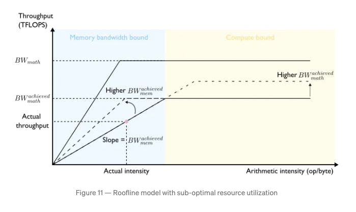
Let's examine a quantitative analysis that applies this model to naive attention.

The analysis is clear: the need to read and write the $\mathcal{O}(N^2)$ matrix to HBM torpedoes the arithmetic intensity, ensuring that performance is dictated by memory bandwidth, not compute power.

3. Solving the Bottleneck: IO-Aware Kernel Fusion

To overcome this, we need an algorithm that avoids materializing the full $(N,N)$ matrix. This is the core innovation of FlashAttention. It is an IO-aware algorithm, meaning it is explicitly designed around the memory hierarchy of the GPU, aiming to minimize data movement between slow HBM and fast on-chip SRAM.

The approach is conceptually similar to the implicit GEMM from our last lesson. It fuses the multiple steps of attention (score calculation, softmax, output calculation) into a single GPU kernel. This kernel computes the final output by loading small blocks (tiles) of the input matrices into the fast SRAM, performing the attention calculation for that block, and updating the output, without ever forming the full $S$ or $P$ matrices in HBM.

This is made possible by two classical techniques applied to attention:

1. Tiling: The computation is broken down into blocks. The kernel iterates through tiles of the Key and Value matrices, computing a portion of the output for a given tile of the Query matrix.
2. Online Softmax: A clever mathematical trick allows the softmax to be computed correctly without having the full row of the $S$ matrix at once. As each new tile is processed, it updates a running maximum and a running sum, allowing it to correctly scale the previous partial results and incorporate the new ones.

Let's delve into these concepts.

Now, let's see how these ideas—tiling and online softmax—are combined to create an efficient, IO-aware algorithm.

4. Analyzing the Optimized Pattern

FlashAttention fundamentally changes the memory access pattern of the attention mechanism.

• Computational Pattern: The total number of FLOPs is actually slightly higher than the naive approach. This is because during the backward pass (for training), the attention scores, which were never saved, must be recomputed. This is a classic speed-memory trade-off: we perform more (cheap) computation to save on (expensive) memory access.
• Memory Access Pattern: This is where the major optimization occurs.
  • The $\mathcal{O}(N^2)$ intermediate matrices are never written to or read from HBM. They exist only ephemerally as small $\mathcal{O}({\text{block\_size}}^2)$ tiles within the fast on-chip SRAM.
  • The memory complexity of the operation is effectively reduced from $\mathcal{O}(N^2)$ to $\mathcal{O}(N)$, as the main memory accesses are just for the Q, K, V, and O matrices.
  • This dramatic reduction in HBM traffic significantly increases the arithmetic intensity, moving the operation from the memory-bound portion of the Roofline model much closer to the compute-bound peak. This allows the GPU's powerful compute units to be utilized much more effectively.

This final clip explains the recomputation strategy.

Conclusion

In this lesson, we dissected the computational and memory access patterns of the Transformer's attention mechanism. We saw how a seemingly straightforward algorithm can lead to severe performance bottlenecks when mapped naively to parallel hardware.

Key Takeaways:

• Standard attention has a computational complexity of $\mathcal{O}(N^{2}d)$ and, more critically, a memory complexity of $\mathcal{O}(N^2)$ due to the need to materialize a large intermediate attention matrix.
• This memory requirement makes the operation memory-bandwidth bound, leading to low GPU utilization as compute units wait for data to be transferred from slow HBM.
• IO-aware algorithms like FlashAttention resolve this by fusing the computational steps into a single kernel that uses tiling to keep working data in fast on-chip SRAM.
• This is enabled by an online softmax formulation, which allows the correct result to be computed without access to the full attention score matrix at once.
• The optimized pattern trades a small increase in computation (via recomputation in the backward pass) for a massive reduction in HBM traffic, resulting in significant speedups and enabling much longer sequence lengths.

Preview of the Next Lesson:

Understanding the performance of a single operation is the first step. To build an efficient system, we must also consider how to execute many computations in parallel. In the next lesson, we will describe how batching strategies affect GPU utilization and throughput in both training and inference, moving from optimizing a single kernel to optimizing the throughput of the entire system.