Convolution as Matrix Multiplication (im2col)

Introduction

Welcome to the next lesson in our module on parallelizing machine learning workloads. In the previous lesson, we dissected the tiled matrix multiplication algorithm, establishing how General Matrix Multiplication (GEMM) is a highly optimized primitive on GPUs, thanks to the effective use of shared memory to manage data locality.

This lesson builds directly on that foundation. The learning outcome is to describe how convolution operations are commonly mapped to matrix multiplication (im2col/implicit GEMM) for GPU efficiency.

You will learn why, instead of being implemented directly, the convolution operation—the workhorse of modern computer vision—is typically transformed into a GEMM operation. We will explore this transformation, known as im2col (image-to-column), and distinguish between a naive, memory-intensive "explicit" approach and the sophisticated "implicit" method used in high-performance libraries like NVIDIA's cuDNN. This understanding is critical for reasoning about the performance of deep learning models on parallel hardware.

1. The Core Idea: Convolution as Matrix Multiplication

At first glance, a convolution seems distinct from a matrix multiplication. It involves a small filter sliding over a larger input tensor, performing element-wise multiplications and summations at each position. However, this series of sliding dot products can be cleverly rearranged into a single, large matrix multiplication. This is the central idea behind the im2col transformation.

The process involves two main steps:

1. Unrolling the Input: The input image or feature map is "unrolled" into a large matrix. Each patch of the input that the filter would slide over becomes a column in this new matrix.
2. Flattening the Filters: The set of convolution filters is flattened into the rows of a second matrix.

Multiplying these two matrices produces a result matrix where each column contains the output values for one spatial location. This output matrix can then be "folded" back into the correct output tensor shape.

This image provides a high-level visual of the transformation:

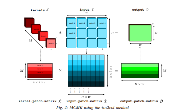
The primary motivation for this transformation is performance. As we saw in the last lesson, GPU hardware and software libraries are exceptionally optimized for GEMM. By converting convolutions to GEMM, we can leverage this massive engineering effort to accelerate our models.

2. Explicit im2col: The Problem of Memory Overhead

A straightforward way to implement this would be to physically create the large unrolled input matrix in the GPU's global memory. This is known as explicit im2col. While conceptually simple, this approach has a major drawback: memory explosion.

Because the sliding windows of the convolution overlap, the same input data element is duplicated many times in the unrolled matrix. For a $K\times K$ filter, each input element can appear up to $K^2$ times. This duplication leads to significant memory overhead and requires a time-consuming data re-organization step before the GEMM can even begin.

The following paper provides a formal introduction to im2col and quantifies the high cost of the explicit approach.

As the paper demonstrates, the explicit method introduces substantial memory and performance penalties, motivating the need for a more sophisticated solution.

3. Implicit GEMM: The Efficient, On-the-Fly Approach

Modern deep learning libraries like cuDNN and PyTorch use a much more elegant solution called implicit GEMM. The core principle is to perform the computation as if the unrolled matrix existed, but without ever fully materializing it in memory. The necessary input data is gathered on-the-fly, directly from the original input tensor, just as it's needed by the GEMM compute units.

This avoids both the memory blow-up and the separate data-copying step of the explicit method. To understand the performance of an implicit GEMM, it's helpful to know the dimensions of the "virtual" matrices being multiplied.

NVIDIA's documentation provides a precise mapping.

A Concrete Mental Model: Manipulating Strides

So, how can we access elements of a "virtual" matrix without creating it? A powerful mechanism for this is the manipulation of memory strides. A stride defines how many bytes to step in memory to get from one element to the next along a given dimension of a tensor. By cleverly defining custom strides, we can create a "view" of the original input tensor that behaves like the unrolled im2col matrix, but without duplicating any data.

The NumPy function as_strided provides an excellent high-level demonstration of this principle. While low-level CUDA kernels don't use NumPy, they employ the same fundamental concept of programmatic address generation based on strides to implement implicit GEMM efficiently.

This technique of creating a logical, strided view of memory is at the heart of how implicit GEMM is realized. It allows the GPU's memory controllers to fetch the correct, non-contiguous data from the original input tensor and feed it to the arithmetic units in the right sequence for the matrix multiplication.

4. Architectural Design Trade-offs

The exact implementation of implicit GEMM involves further architectural trade-offs. The paper you read earlier, "Characterizing and Demystifying the Implicit Convolution Algorithm," proposes a specific strategy called channel-first im2col.

Let's briefly touch on the core idea, as it exemplifies the kind of architectural reasoning involved in designing high-performance systems.

• Traditional (channel-last) im2col: Conceptually orders the unrolled matrix by first iterating through all channels for a given filter position (e.g., C -> H -> W). This can lead to complex data access patterns for the hardware.
• Proposed (channel-first) im2col: Reorders the "virtual" columns of the matrix to group all data for a specific filter position across all output locations (e.g., H -> W -> C).

The paper argues that this reordering results in a simpler and more efficient data access pattern for hardware like TPUs and GPUs. It allows data to be read in contiguous chunks (all channels for a single pixel (h, w)) and simplifies the address generation logic.

This discussion of channel-first vs. channel-last layouts highlights a key theme in systems design: the interplay between algorithm design (the im2col transformation) and hardware architecture (memory layout, data path). The optimal solution is one where the software's data access patterns align with the hardware's strengths.

Conclusion

In this lesson, we have bridged the gap between the highly optimized GEMM primitive and the ubiquitous convolution operation. By transforming convolutions into matrix multiplications, deep learning frameworks unlock the full power of modern GPUs.

Key Takeaways:

• Convolutions are mapped to GEMM on GPUs because GEMM is an exceptionally well-optimized operation.
• The im2col transformation unrolls input tensor patches into columns of a matrix, allowing the convolution to be computed as a single GEMM.
• Explicit im2col materializes the unrolled matrix, incurring significant memory and performance overhead due to data duplication.
• Implicit GEMM is the modern approach used in libraries like cuDNN. It computes the GEMM on "virtual" matrices that are never stored in memory, generating the required data on-the-fly by manipulating memory strides and addresses.
• The specific implementation of implicit GEMM involves architectural trade-offs, such as the choice of data layout (channel-first vs. channel-last), to best align with the underlying hardware's capabilities.

Preview of the Next Lesson:

Now that we have established how fundamental operations like GEMM and convolution are parallelized, we will turn our attention to more complex components. In the next lesson, we will analyze the computational and memory access patterns of the attention mechanism in Transformers, another critical building block of modern AI that presents unique challenges for GPU acceleration.