Operator Fusion for Performance

Introduction

Welcome to the next lesson in our exploration of how machine learning workloads are optimized for GPU hardware. In our previous sessions, we've tackled optimization from two different angles. We went deep into a single kernel with FlashAttention, seeing how algorithmic changes can drastically reduce memory I/O. Then, we zoomed out to the system level with batching, understanding how to group work to maximize GPU throughput. A common thread has been the constant battle against the "memory wall"—the bottleneck created by moving data between the GPU's vast but slow global memory (HBM) and its small but fast on-chip memory (SRAM and registers).

Today, we'll explore a crucial compiler optimization that directly attacks this problem: operator fusion. This lesson addresses the learning outcome: Explain the role of operator fusion in reducing memory traffic and improving kernel performance. We will investigate how ML compilers like XLA and TVM automatically rewrite your computation graph, merging multiple simple operations into a single, more efficient GPU kernel. This technique is fundamental to achieving high performance in frameworks like PyTorch and TensorFlow.

1. The Core Problem: Memory Round-Trips and Kernel Overhead

At a high level, a neural network is a directed acyclic graph (DAG) of operations. A naive execution strategy would be to launch a separate GPU kernel for each node in the graph. For example, a Conv -> BiasAdd -> ReLU sequence would involve three separate kernel launches.

This approach suffers from two primary sources of inefficiency:

1. Kernel Launch Overhead: Each time the CPU instructs the GPU to launch a kernel, there is a non-trivial overhead. This involves driver calls, command buffer submissions, and context switching. For a graph with thousands of small operations, this overhead can become a significant portion of the total execution time.

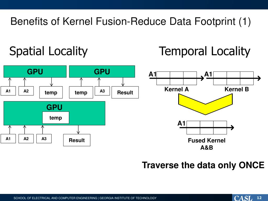
2. Memory Traffic: This is the far more critical issue. In the Conv -> BiasAdd -> ReLU example, the naive approach would be:

   • Kernel 1 (Conv): Reads inputs from global memory, performs computation, and writes the intermediate result back to global memory.
   • Kernel 2 (BiasAdd): Reads the intermediate result from global memory, adds the bias, and writes a new intermediate result back to global memory.
   • Kernel 3 (ReLU): Reads the second intermediate result from global memory, applies the activation, and writes the final output to global memory.

The intermediate tensors are written to and read from slow HBM, creating unnecessary memory traffic. Operator fusion is a compiler optimization that avoids this by combining these sequential operations into a single, monolithic kernel.

Let's watch a short, clear explanation of this concept from a talk on ML compilers.

As the video highlights, fusion fundamentally trades increased on-chip computation and code complexity for a significant reduction in off-chip memory access. Given that memory bandwidth is often the primary bottleneck, this is almost always a worthwhile trade.

2. The Anatomy of Fusion: Vertical and Horizontal

Operator fusion strategies are typically categorized into two main types based on the structure of the graph they optimize.

Let's break down these two types:

Vertical Fusion (Producer-Consumer)

This is the most common type of fusion, combining operations that form a sequential chain in the computation graph. The output of one operator is the input to the next.

• Example: Conv2D -> BiasAdd -> ReLU
• Without Fusion: 3 kernels, 2 intermediate tensors written to/read from HBM.
• With Fusion: 1 kernel. The result of the convolution is kept in on-chip registers, the bias is added, the ReLU is applied, and only the final result is written to HBM.
• Benefit: Eliminates intermediate memory round-trips and reduces kernel launch overhead.

Horizontal Fusion

This type of fusion combines parallel operations that are independent of each other but consume the same input tensor.

• Example: Projecting an input tensor x to Query, Key, and Value in a Transformer: x -> MatMul_Q, x -> MatMul_K, x -> MatMul_V.
• Without Fusion: 3 separate MatMul kernels, each reading the tensor x from HBM.
• With Fusion: The weight matrices for Q, K, and V are concatenated, and a single, larger MatMul kernel is executed.
• Benefit: The input tensor x is read from HBM only once. A secondary benefit is that a single larger kernel often achieves better GPU occupancy and efficiency than three smaller ones.

3. The Compiler's Dilemma: To Fuse or Not to Fuse?

While fusion is powerful, blindly fusing all possible operations can hurt performance. An effective ML compiler must make intelligent decisions based on a cost model. This is an area where your background in algorithms and optimization is highly relevant. The compiler is essentially solving an optimization problem: find the graph partitioning (i.e., the set of fused kernels) that minimizes the predicted execution time.

As the article details, a compiler's cost model must weigh several factors:

• Benefit of fusion:
  • Reduced memory I/O (often the biggest win).
  • Reduced kernel launch overhead.
  • Improved data locality and cache utilization.
• Cost of fusion:
  • Increased Register Pressure: A fused kernel performs more work and must hold more intermediate values simultaneously. If the number of live variables exceeds the available registers per thread, the compiler must "spill" them to a slower memory tier (like L1 cache or even global memory), which can negate the benefits of fusion.
  • Re-computation: As seen in the Stanford video, if a node has multiple consumers, fusing it with one may require it to be recomputed for the other. The cost model must decide if re-computing is cheaper than storing the intermediate result.
  • Code Complexity & Instruction Cache: Very large, complex fused kernels can potentially lead to instruction cache misses, slowing down the GPU's fetch-and-decode pipeline.

The compiler uses this model to evaluate candidate fusions, accepting a fusion only if the predicted cost is lower than the unfused alternative. Modern ML compilers like Google's XLA and NVIDIA's TensorRT have highly sophisticated, hardware-specific cost models to make these decisions.

4. A Structured Approach: Fusion Rules

To manage this complexity, compilers don't just randomly try to fuse nodes. They categorize operators and apply a set of rules. While the details are complex, we can understand the high-level logic.

The "Operator Fusion Strategies" article (LINK) that we read earlier briefly introduced these categories under the heading "Fusion Rules and Topological Constraints." Let's revisit that concept:

• Injective (Element-wise): One-to-one mapping (e.g., Add, ReLU). These are the easiest to fuse.
• Reduction: Many-to-one mapping (e.g., Sum, MaxPool). Fusing an element-wise op into a reduction is common (e.g., apply ReLU then sum). Fusing a reduction into something else is harder.
• Broadcast: One-to-many mapping (e.g., adding a vector to a matrix).
• Opaque: Complex operations the compiler cannot analyze (e.g., Sort). These act as "fusion barriers," forcing the compiler to end one fused kernel and start another.

A typical fusion algorithm traverses the graph, greedily merging compatible nodes based on these classifications and the cost model's guidance, stopping whenever it hits an opaque operator or a fusion that the cost model deems unprofitable.

Conclusion

In this lesson, we dissected operator fusion, a critical compiler optimization that sits at the intersection of graph theory, hardware architecture, and performance modeling. It is a prime example of how modern ML systems bridge the gap between a high-level model definition and efficient execution on parallel hardware.

Key Takeaways:

• Operator fusion mitigates the memory bandwidth bottleneck by merging multiple operations into a single GPU kernel.
• This reduces two main overheads: kernel launch costs and, more importantly, intermediate memory round-trips to and from global memory.
• The primary strategies are vertical fusion (for sequential producer-consumer patterns) and horizontal fusion (for parallel operations with a shared input).
• The decision to fuse is not always straightforward. Compilers use a sophisticated cost model to weigh the benefits (reduced memory I/O) against potential costs (increased register pressure, re-computation).
• By increasing the ratio of arithmetic operations to memory accesses (arithmetic intensity), fusion helps move workloads from being memory-bound to being compute-bound, allowing the GPU to operate closer to its peak performance.

Preview of the Next Lesson:

So far, we have focused on optimizing computation and data movement using full-precision (FP32) numbers. However, the hardware itself offers another powerful lever for optimization. In our next lesson, we will explore how to further improve performance by changing the data itself. We will cover the final topic of this module: "Explain how mixed-precision training (FP16/BF16) with dynamic loss scaling reduces memory footprint and leverages Tensor Cores." This will connect directly to our discussion of specialized hardware from the first module.