Mixed-Precision Training: Memory Efficiency and Tensor Core Utilization

Introduction

Welcome to our final lesson in the module on parallelizing machine learning workloads. In our previous lesson, we explored operator fusion, a compiler optimization that rewrites the computation graph to reduce memory traffic and kernel launch overhead. We saw how this technique helps bridge the performance gap between a high-level model definition and the underlying hardware by making better use of on-chip memory.

Today, we take this a step further. Instead of just rearranging computations, we will investigate how changing the numerical format of the data itself can unlock significant performance gains. This lesson addresses the learning outcome: Explain how mixed-precision training (FP16/BF16) with dynamic loss scaling reduces memory footprint and leverages Tensor Cores.

We will cover:

1. The two primary benefits of using lower-precision formats: reduced memory usage and access to specialized hardware accelerators.
2. The characteristics of 16-bit floating-point formats, FP16 and BF16, and their trade-offs compared to the standard 32-bit FP32.
3. The critical techniques—maintaining FP32 master weights and dynamic loss scaling—required to maintain numerical stability and ensure successful training.

1. The Motivation: Why Use Lower Precision?

For years, FP32 (single precision) was the default data type for training deep neural networks. However, as models grew larger, the computational and memory costs became prohibitive. This prompted a move towards using lower-precision formats, primarily for two reasons.

Benefit 1: Reduced Memory Footprint and Bandwidth

The most direct benefit of switching from 32-bit to 16-bit numbers is that every value now takes up half the space. This has a cascading effect throughout the training process:

• Model Parameters: A model with 10 billion parameters would require 40 GB in FP32, but only 20 GB in FP16.
• Activations: Intermediate activations, which are stored between the forward and backward passes, also see their memory footprint halved. This is often the largest consumer of GPU memory.
• Gradients: Gradients computed during backpropagation are also halved in size.

This memory saving allows you to either train larger models that would otherwise not fit on a single GPU or use larger batch sizes, which can improve hardware utilization and sometimes lead to faster convergence. Furthermore, since data transfers are a major bottleneck, moving half the amount of data between the GPU's main memory (HBM) and its compute units reduces memory bandwidth pressure.

Benefit 2: Specialized Hardware Acceleration with Tensor Cores

Modern NVIDIA GPUs (since the Volta architecture) include specialized hardware units called Tensor Cores. These are distinct from the standard CUDA cores (which are general-purpose FP32 ALUs) and are explicitly designed to accelerate matrix multiply-accumulate (MMA) operations, which are the heart of convolutions and linear layers.

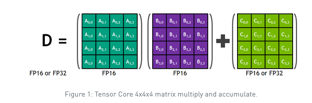
Tensor Cores operate on 16-bit inputs (FP16 or BF16) but can accumulate the results in higher precision (FP32). This design provides a massive increase in theoretical throughput—up to 8x or more compared to FP32 operations on the same GPU. By using 16-bit formats, you enable the ML framework's kernels to leverage these powerful accelerators.

2. A Look at Floating-Point Formats: FP32 vs. FP16 vs. BF16

To understand the trade-offs of mixed-precision training, we must first understand the data formats themselves. A floating-point number is typically represented by a sign bit, an exponent, and a mantissa (or fraction). The number of bits allocated to the exponent determines the range of representable numbers, while the bits for the mantissa determine the precision (the "fineness" of the numbers within that range).

• FP32 (Single Precision): 1 sign bit, 8 exponent bits, 23 mantissa bits. This is the standard baseline, offering a wide range and high precision.
• FP16 (Half Precision): 1 sign bit, 5 exponent bits, 10 mantissa bits. Compared to FP32, it has a drastically smaller range, making it susceptible to numbers becoming too large (overflow) or too small (underflow).
• BF16 (Brain Floating-Point): 1 sign bit, 8 exponent bits, 7 mantissa bits. Developed by Google, this format keeps the same 8-bit exponent as FP32, giving it a comparable dynamic range. The trade-off is a significantly reduced mantissa, leading to lower precision (more rounding errors).

The following video provides an excellent, detailed explanation of these formats and their trade-offs.

To summarize the key trade-off:

• FP16 is more precise than BF16 but has a very narrow dynamic range, making it prone to underflow and overflow issues.
• BF16 has the same dynamic range as FP32 (making it numerically more stable) but sacrifices precision, which can affect the model's ability to converge on some tasks.

3. Making it Work: The Challenges of 16-Bit Training

Simply casting all operations to FP16 and hoping for the best often leads to failed training. The limited range and precision of FP16 introduce two critical numerical stability problems.

Problem 1: Inaccurate Weight Updates

During training, the update applied to a weight is typically very small ($\Delta w=\eta \cdot \nabla L$). If the weight itself is relatively large and stored in FP16, adding this tiny update might result in no change at all due to the limited precision of the 16-bit mantissa. The update gets rounded to zero, and the weight stops learning.

Solution: Maintain an FP32 Master Copy of Weights

The standard solution is to perform the forward and backward passes using an FP16 copy of the weights to get the performance benefits. However, a master copy of the weights is maintained in full FP32. After the FP16 gradients are computed, they are used to update this FP32 master copy, which has enough precision to accumulate the tiny updates over time. A fresh FP16 copy is then created from the updated master weights for the next iteration.

Problem 2: Gradient Underflow

The second major issue, particularly for FP16, is its limited dynamic range. During backpropagation, gradient values can become extremely small. If they fall below the minimum representable positive value for FP16 (~6.10e-5), they are "flushed" to zero. This is known as gradient underflow. When this happens, the gradient signal is lost, and the corresponding weights are not updated, effectively halting training for parts of the network.

Solution: Loss Scaling

The solution is to artificially "shift" the gradient values into the representable range of FP16. This is done by scaling the loss up by a large scaling factor, $S$, before backpropagation begins.

$$\text{scaled\_loss}=\text{loss}\cdot S$$

By the chain rule of differentiation, all the gradients will also be scaled by $S$:

$$\frac{\partial (\text{loss}\cdot S)}{\partial w}=S\cdot \frac{\partial \text{loss}}{\partial w}$$

This scaling pushes the small gradient values out of the underflow region and into the representable range of FP16. Before the weight update is applied to the FP32 master weights, the gradients are scaled back down by dividing by $S$, restoring their original values.

Dynamic Loss Scaling

Choosing a fixed scaling factor $S$ can be difficult. If it's too small, underflow still occurs. If it's too large, the scaled gradients might overflow (become Inf or NaN). A more robust approach is dynamic loss scaling:

1. Start with a large scale factor $S$.
2. After each backpropagation step, check the gradients for Inf or NaN values.
3. If an overflow is detected, skip the weight update for that step and decrease $S$ (e.g., by half).
4. If no overflow occurs for a certain number of consecutive steps, increase $S$ (e.g., by double).

This algorithm automatically finds the largest possible scaling factor that avoids overflow, maximizing the preservation of small gradient values.

4. Putting It All Together: Automatic Mixed Precision (AMP)

Manually implementing these techniques—casting certain ops to FP16, maintaining FP32 master weights, and managing dynamic loss scaling—is complex and error-prone. Fortunately, modern deep learning frameworks provide Automatic Mixed Precision (AMP) libraries that handle all of this for you.

With AMP, you typically only need to add a few lines of code to your training script. The library will then automatically:

• Identify which operations can be safely run in FP16 to leverage Tensor Cores (e.g., convolutions, matrix multiplies).
• Keep operations that require higher precision in FP32 (e.g., reductions, loss functions).
• Manage the creation and updating of FP32 master weights.
• Apply dynamic loss scaling.

The overall workflow looks like this:

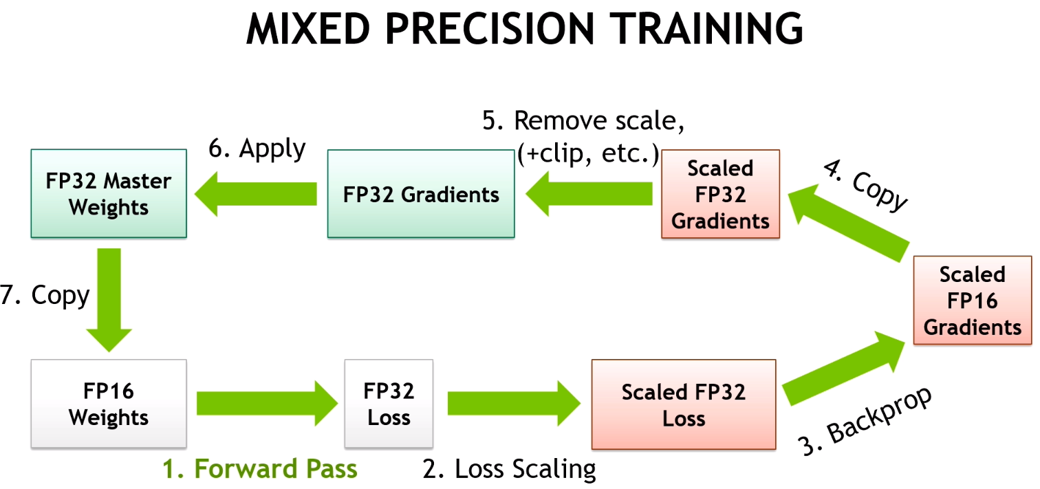
This automation makes mixed-precision training accessible and is a standard feature for achieving high performance in deep learning today.

Conclusion

In this lesson, we have uncovered how mixed-precision training serves as a powerful optimization strategy, attacking both memory and compute limitations simultaneously. It demonstrates a key principle in high-performance computing: tailoring your data representation and algorithms to the specific capabilities of the underlying hardware.

Key Takeaways:

• Mixed-precision training combines 16-bit (FP16/BF16) and 32-bit (FP32) floating-point formats to accelerate training.
• The primary benefits are reduced memory footprint (allowing for larger models/batches) and higher computational throughput by leveraging specialized hardware like Tensor Cores.
• Using 16-bit formats presents numerical stability challenges, namely inaccurate weight updates and gradient underflow.
• These challenges are overcome by maintaining an FP32 master copy of weights for updates and applying dynamic loss scaling to prevent small gradients from being flushed to zero.
• Frameworks like PyTorch and TensorFlow offer Automatic Mixed Precision (AMP) utilities that automate this entire process, making it easy to implement.

Preview of the Next Lesson and Module:

This lesson concludes our module on parallelizing workloads on a single GPU. We've seen how to parallelize matrix operations, optimize data access patterns with operator fusion, and now, how to leverage lower-precision arithmetic.

The next logical step is to scale beyond a single device. Our next module, "Multi-GPU Communication: Interconnects and Collectives," will explore how to train models that are too large or take too long to train on one GPU. We will begin by examining the physical hardware that connects GPUs together, comparing intra-node interconnects like PCIe and NVLink.