Calculating MIRR with Explicit Reinvestment

Hello! Welcome to your next lesson in our module on "Advanced Performance and Risk-Adjusted Returns."

In the previous lesson, we explored the equity multiple, a metric that tells us the total magnitude of our return but ignores the time value of money. We contrasted this with the IRR, which is highly sensitive to the timing of cash flows. However, IRR has a significant, often misunderstood, flaw in its underlying assumptions. This lesson will introduce a metric designed to fix that flaw.

Today's learning outcome is to compute the modified internal rate of return (MIRR) with explicit reinvestment assumptions. The MIRR provides what many consider a more realistic annualized rate of return by allowing you to explicitly state what you'll do with cash flows generated during the investment's life.

1. The Core Problem with the Internal Rate of Return (IRR)

Before we can appreciate MIRR, we must first understand the primary critique of the traditional IRR. As a quick refresher, the IRR is the discount rate that makes the Net Present Value (NPV) of all cash flows from a project equal to zero.

The critical, and often unrealistic, assumption embedded within the IRR calculation is that all interim positive cash flows generated by the project are reinvested at the IRR itself.

Imagine a project has an IRR of 25%. The formula implicitly assumes that any cash you receive in Year 1, Year 2, etc., can be immediately put into another investment that also yields 25% for the remainder of the holding period. In most market conditions, finding subsequent opportunities with such a high rate of return is highly unlikely. This assumption often leads to an overestimation of the project's true profitability.

The following video provides an excellent explanation of this problem and sets the stage for why a "modified" IRR is necessary.

As the video explains, this flawed assumption can lead to poor capital budgeting decisions. A project may look fantastic on paper with a 77% IRR, but if the actual achievable reinvestment rate is closer to 10%, the real-world return will be drastically lower.

2. Introducing the Modified Internal Rate of Return (MIRR)

The Modified Internal Rate of Return (MIRR) directly addresses this reinvestment problem. Instead of implicitly assuming cash flows are reinvested at the IRR, MIRR allows you to specify two distinct, explicit rates:

1. Reinvestment Rate: The rate at which you assume positive cash flows from the investment can be reinvested until the end of the holding period. This is typically a more conservative and realistic rate, such as your cost of capital, the interest rate on a savings account, or the expected return of a broad market index.
2. Financing Rate: The rate at which you can borrow funds to cover any negative cash flows (e.g., for capital expenditures) that occur after the initial investment. This is often your borrowing cost or the rate on a line of credit.

By separating these rates, MIRR provides a more accurate and defensible measure of a project's long-term, compound annual return.

3. The MIRR Calculation: A Step-by-Step Guide

The calculation of MIRR can be broken down into three logical steps:

Step 1: Calculate the Present Value of Outflows (PVO)
Discount all negative cash flows (your initial investment and any future capital calls) to Year 0 using the financing rate. This gives you a single value representing the total investment in today's euros.
$\text{PVO}={\sum }_{t=0}^n\frac{{\text{CashOutflow}}_t}{(1+\text{FinancingRate}{)}^t}$
(Note: Outflows are treated as positive values in this formula for simplicity).

Step 2: Calculate the Future Value of Inflows (FVI)
Compound all positive cash flows (from operations and sale) forward to the end of the holding period using the reinvestment rate. This gives you a single "terminal value" representing the total cash you'll have at the end.
$\text{FVI}={\sum }_{t=0}^n{\text{CashInflow}}_t\times (1+\text{ReinvestmentRate}{)}^{n-t}$

Step 3: Calculate the MIRR
The MIRR is the compound annual growth rate that grows the PVO into the FVI over the holding period (n). The formula is:
$\text{MIRR}={\left(\frac{\text{FVI}}{\text{PVO}}\right)}^{\frac{1}{n}}-1$

This process transforms a complex stream of cash flows into a simple time value of money problem: "I invested PVO today and ended up with FVI in n years. What was my annual rate of return?"

The following video walks through this manual calculation with a clear example.

4. A Spanish Real Estate Example

Let's apply this to a property investment scenario with some non-conventional cash flows.

Scenario:

• Initial Investment (Year 0): -€200,000
• Annual Net Cash Flow (Years 1-2): €12,000
• Capital Expenditure for renovation (Year 3): -€25,000
• Annual Net Cash Flow (Years 4-5): €18,000 (higher rent post-renovation)
• Net Sale Proceeds (end of Year 5): €280,000
• Holding Period (n): 5 years

Assumptions for MIRR:

• Financing Rate: 4% (cost to borrow for the renovation)
• Reinvestment Rate: 7% (expected return from a conservative investment portfolio)

Let's calculate:

Step 1: PVO (at 4% financing rate)
The only outflow after Year 0 is the €25,000 in Year 3.
$\text{PVO}=€200,000+\frac{€25,000}{(1+0.04{)}^3}=€200,000+\frac{€25,000}{1.12486}=€200,000+€22,225=€222,225$

Step 2: FVI (at 7% reinvestment rate)
The positive cash flows are in years 1, 2, 4, and 5. The final cash flow in year 5 is €18,000 + €280,000 = €298,000.

$$\begin{array}{rl}\text{FVI}=& (€12,000\times (1.07{)}^4)+(€12,000\times (1.07{)}^3)+(€18,000\times (1.07{)}^1)+€298,000\\ \text{FVI}=& (€12,000\times 1.3108)+(€12,000\times 1.2250)+(€18,000\times 1.07)+€298,000\\ \text{FVI}=& €15,730+€14,700+€19,260+€298,000=€347,690\end{array}$$

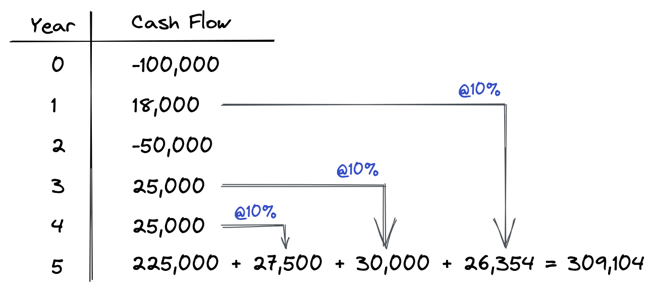
Step 3: Calculate MIRR
$\text{MIRR}={\left(\frac{€347,690}{€222,225}\right)}^{\frac{1}{5}}-1=(1.5646{)}^{\frac{1}{5}}-1=1.0936-1=9.36\%$

The standard IRR for this same set of cash flows is 10.87%. As expected, the MIRR provides a more conservative and likely more realistic rate of return by tempering the reinvestment assumption.

Test your understanding!

An investment has the following cash flows:

• Year 0: -€150,000
• Year 1: €15,000
• Year 2: €15,000
• Year 3: €15,000 + €190,000 (sale) = €205,000

Assume a reinvestment rate of 5% and a financing rate of 3%. There are no negative cash flows after Year 0. Calculate the MIRR.

Show answer

1. PVO: Since the only outflow is at Year 0, PVO = €150,000.
2. FVI:
   • FV of Year 1 cash flow: €15,000 * (1.05)^2 = €16,537.50
   • FV of Year 2 cash flow: €15,000 * (1.05)^1 = €15,750.00
   • Year 3 cash flow (already at end): €205,000.00
   • Total FVI = €16,537.50 + €15,750.00 + €205,000.00 = €237,287.50
3. MIRR:
   • MIRR = (€237,287.50 / €150,000)^(1/3) - 1
   • MIRR = (1.5819)^(1/3) - 1 = 1.165 - 1 = 16.5%

5. Coding MIRR in Python

As a software engineer, you'll appreciate that libraries exist to handle this calculation. The numpy_financial package, which you may already have from our previous coding exercises, includes a handy mirr function.

The function signature is numpy_financial.mirr(values, finance_rate, reinvest_rate).

Let's implement our Spanish real estate example from section 4 in Python.

import numpy_financial as npf

# Cash flows from the example in section 4
# Negative values for outflows, positive for inflows
cash_flows = [-200_000, 12_000, 12_000, -25_000, 18_000, 18_000 + 280_000]

# Rates
finance_rate = 0.04
reinvest_rate = 0.07

# Calculate MIRR using numpy_financial
mirr_value = npf.mirr(cash_flows, finance_rate, reinvest_rate)

# Calculate IRR for comparison
irr_value = npf.irr(cash_flows)

print(f"The cash flows are: {cash_flows}")
print(f"Financing Rate: {finance_rate:.2%}")
print(f"Reinvestment Rate: {reinvest_rate:.2%}")
print("-" * 30)
print(f"Calculated MIRR: {mirr_value:.2%}")
print(f"Calculated IRR: {irr_value:.2%}")

# The Python output for MIRR is 9.36%, matching our manual calculation.

This demonstrates how easily you can integrate this more robust metric into your financial models.

Conclusion

Today we've delved into one of the most important critiques of IRR and learned how to use a superior metric, the MIRR.

Key Takeaways:

• The Internal Rate of Return (IRR) implicitly assumes interim cash flows are reinvested at the IRR itself, which can significantly overstate returns.
• The Modified Internal Rate of Return (MIRR) solves this by using explicit, user-defined rates: a financing rate for outflows and a reinvestment rate for inflows.
• The MIRR calculation involves finding the present value of all costs, the future terminal value of all returns, and then solving for the equivalent annual rate.
• MIRR almost always provides a more conservative, and arguably more realistic, measure of an investment's compound annual return compared to IRR. It also solves the "multiple IRR" problem for non-conventional cash flows.

Preview of the Next Lesson:
Both IRR and MIRR are percentage rates, which are great for comparing efficiency but don't tell us about the scale of value creation. In our next lesson, we will learn how to calculate the Profitability Index (PI). This metric brings us back to NPV and provides a ratio that measures the value created per euro invested, making it an excellent tool for comparing investment opportunities of different sizes.