Equity Multiple Calculation

Hello! Welcome to the first lesson in our module on "Advanced Performance and Risk-Adjusted Returns."

In the previous module, we concluded by building a comprehensive Discounted Cash Flow (DCF) model in Python. That exercise was all about determining a property's intrinsic value. Now, we pivot from valuation to performance. Instead of asking "What is this property worth?", we'll start asking, "How good of an investment is this property?"

Our first step in answering that question is to master a simple yet fundamental metric: the equity multiple. The learning outcome for this lesson is to calculate the equity multiple to evaluate the total cash return to the investor. This metric answers the straightforward question: for every euro I put into this deal, how many euros do I get back in total over the entire life of the investment?

1. What is the Equity Multiple?

The equity multiple is one of the most intuitive metrics in real estate. It measures the total cash returned to an investor relative to the total equity they invested. It's often referred to as the Multiple on Invested Capital (MOIC) in other areas of finance.

The formula is simple:

$\text{Equity Multiple}=\frac{\text{Total Cash Distributions}}{\text{Total Equity Invested}}$

• Total Cash Distributions: This includes all cash flow received from the property during the holding period (e.g., annual pre-tax cash flow) PLUS the net cash received from the sale of the property at the end.
• Total Equity Invested: This is the initial down payment plus any subsequent capital contributions made by the investor during the holding period.

To get a clear definition and see a simple example, the following article is a great starting point.

2. Calculation and Interpretation

Let's illustrate with a practical example. Imagine you invest in a property with the following cash flows over a 5-year hold:

• Initial Equity Investment (Year 0): €100,000
• Annual Cash Flow (Years 1-4): €5,000 per year
• Annual Cash Flow (Year 5): €5,000
• Net Sale Proceeds (Year 5): €180,000

Let's calculate the components:

1. Total Equity Invested: €100,000
2. Total Cash Distributions:
   • Cash flow from operations: (4 years * €5,000) + €5,000 = €25,000
   • Cash from sale: €180,000
   • Total: €25,000 + €180,000 = €205,000

Now, we apply the formula:

$\text{Equity Multiple}=\frac{€205,000}{€100,000}=2.05x$

This means for every euro you invested, you received €2.05 back over the life of the investment.

The image below, from the Wall Street Prep article, shows a similar calculation in a familiar spreadsheet format.

So, what makes a "good" equity multiple? Here’s a simple guide:

• Equity Multiple < 1.0x: You received less money back than you put in. A loss.
• Equity Multiple = 1.0x: You broke even. You got back exactly what you invested.
• Equity Multiple > 1.0x: You made a profit. You recovered your initial investment and received an additional return.

3. The Power and Pitfalls of the Equity Multiple

You might be thinking, "This is much simpler than IRR or NPV. Why is it considered an 'advanced' metric?" The power of the equity multiple lies not in its complexity, but in its use as a sanity check alongside more sophisticated, time-sensitive metrics like the Internal Rate of Return (IRR).

The key weakness of the equity multiple is that it completely ignores the time value of money. A 2.0x multiple achieved in 2 years is vastly superior to a 2.0x multiple achieved in 10 years, but the metric itself doesn't show that difference.

Conversely, IRR's focus on the timing of cash flows can sometimes be misleading. A short-term project with a quick flip can generate a very high IRR, but the actual profit in dollar terms (and thus the equity multiple) might be quite low. A longer-term project might have a lower IRR but generate a much larger total return on capital.

The following video explains this crucial relationship brilliantly.

As the video highlights, many sophisticated investors require a deal to meet both an IRR hurdle and an equity multiple hurdle to ensure they are compensated for both the speed and the magnitude of their return.

Test your understanding!

Look at the image below which shows two different investments.

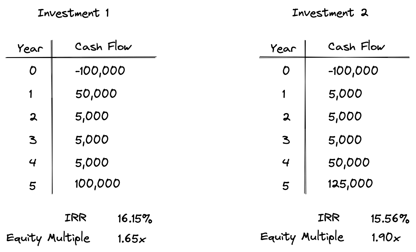
Which investment would you prefer and why? Justify your answer by referencing both the IRR and the Equity Multiple.

Show answer

There's no single "right" answer; it depends on your investment goals.

• Argument for Investment 1: It has a slightly higher IRR (16.15% vs. 15.56%), meaning it generates returns more efficiently over time. If your primary goal is to recycle capital quickly into new deals, a higher IRR might be preferable.
• Argument for Investment 2: It has a significantly higher Equity Multiple (1.90x vs. 1.65x). If your goal is to maximize the total amount of profit from your initial capital, this is the better choice. You put in €100,000 and get €190,000 back, versus getting €165,000 back from Investment 1.

This perfectly illustrates the trade-off: IRR measures the rate of return, while Equity Multiple measures the magnitude of the return.

4. Calculating the Equity Multiple in Python

Given your background, let's create a simple Python function to calculate this. This function will build on the cash flow concepts from our DCF model. It will take two lists: one for all cash outflows (investments) and one for all cash inflows (distributions).

import numpy as np

def calculate_equity_multiple(
    equity_contributions: list[float], 
    cash_distributions: list[float]
) -> float:
    """
    Calculates the equity multiple for an investment.

    Args:
        equity_contributions (list[float]): A list of all cash outflows (as positive numbers).
                                            e.g., [100000, 20000] for a down payment and a later capital call.
        cash_distributions (list[float]): A list of all cash inflows from operations and sale.
                                          e.g., [5000, 5000, 205000]

    Returns:
        float: The calculated equity multiple, or 0 if no equity was contributed.
    """
    total_equity_invested = sum(equity_contributions)
    total_cash_distributed = sum(cash_distributions)

    if total_equity_invested <= 0:
        return 0.0

    equity_multiple = total_cash_distributed / total_equity_invested
    return equity_multiple

# --- Example Usage ---

# Scenario 1: Simple case from section 2
initial_investment = [100_000]
op_cash_flow = [5_000] * 5
sale_proceeds = [180_000]
# In year 5, you get both the final operating cash flow and the sale proceeds.
# For simplicity, we can list them all.
all_distributions_1 = [5_000, 5_000, 5_000, 5_000, 5_000 + 180_000]

em_1 = calculate_equity_multiple(initial_investment, all_distributions_1)
print(f"Scenario 1 Equity Multiple: {em_1:.2f}x")

# Scenario 2: A deal with a later capital call
investments_2 = [100_000, 25_000] # Initial investment + capital call in Year 2 for renovations
distributions_2 = [6_000, 6_000, 10_000, 10_000, 10_000 + 250_000] # Higher cash flow and sale price

em_2 = calculate_equity_multiple(investments_2, distributions_2)
print(f"Scenario 2 Equity Multiple: {em_2:.2f}x")

This simple function correctly handles cases with single or multiple equity contributions, a crucial nuance for realistic deal analysis.

Conclusion

In this lesson, you've learned how to calculate and interpret the equity multiple, a core metric for assessing the overall profitability of an investment.

Key Takeaways:

• Equity Multiple is the ratio of Total Cash Distributions to Total Equity Invested.
• It provides a simple, intuitive measure of how many times you get your money back. A multiple of 2.5x means you received €2.50 for every €1.00 invested.
• Its main strength is its simplicity and focus on total profit magnitude.
• Its main weakness is its disregard for the time value of money, making it essential to use it alongside metrics like IRR and NPV, not in isolation.

Preview of the Next Lesson:
We've established that the equity multiple ignores time, while IRR can sometimes be misleading. Is there a metric that tries to find a middle ground? In our next lesson, we will explore the Modified Internal Rate of Return (MIRR). You'll learn how MIRR addresses some of IRR's theoretical flaws by using explicit assumptions about reinvestment rates, providing what many consider a more realistic measure of a project's long-term, annualized return.