Marginal Cost and Marginal Product: An Inverse Relationship

Introduction

Hello! Welcome back to our study of production costs. In our last few lessons, you’ve become familiar with two very important concepts:

1. From our lesson on production, you learned about the marginal product of labor (MP) and the law of diminishing marginal returns, which gives the MP curve its characteristic "hill" shape.
2. In our most recent lesson, you learned to graph the marginal cost (MC) curve and saw that it typically has a "U" shape.

As I hinted at the end of our last session, the fact that the MP curve is shaped like a hill and the MC curve is shaped like a U is no coincidence. They are, in fact, two sides of the same coin.

Today's lesson directly addresses the learning outcome: to explain the relationship between the marginal cost curve and the marginal product curve. We will formally connect a firm's production technology (what it gets from its workers) to its cost structure (what it costs to produce more output). This connection is fundamental to understanding how firms make decisions.

1. The Core Relationship: Productivity and Cost

The link between marginal product and marginal cost is intuitive. Think about it from a firm's perspective:

• When you hire a new worker and they are highly productive (i.e., they have a high marginal product), they add a lot of output for the cost of their wage. This means the cost of producing each of those additional units is low.
• Later, due to diminishing returns, a new worker you hire is less productive (they have a low marginal product). You still pay them the same wage, but they add less output. This means the cost of producing each of those few additional units is high.

In short:

• Increasing marginal product leads to decreasing marginal cost.
• Diminishing (decreasing) marginal product leads to increasing marginal cost.

This creates the inverse, or "mirror image," relationship between the two curves.

2. Seeing it in Action: An Intuitive and Numerical Explanation

Let's watch a short video that brings this concept to life. It starts with the core intuition and then walks through a clear numerical example to prove the relationship.

3. The Formal Relationship: A Simple Equation

The video demonstrated this inverse relationship with numbers. We can formalize this with a simple but powerful formula.

Remember that marginal cost is the change in total cost divided by the change in quantity:
$MC=\frac{\Delta TC}{\Delta Q}$

In the short run, when a firm hires more labor to produce more output, the change in total cost ($\Delta TC$) is the cost of the additional labor, which is the wage ($w$) paid to the new worker(s). The change in quantity ($\Delta Q$) is the additional output they produce, which is their marginal product ($MP$).

If we consider hiring just one more unit of labor, the formula becomes:
$MC=\frac{w}{MP}$

This equation makes the inverse relationship crystal clear. Since the wage ($w$) is a constant price for the input, if Marginal Product ($MP$) in the denominator goes up, Marginal Cost ($MC$) must go down. Conversely, when $MP$ goes down (due to diminishing returns), $MC$ must go up.

To confirm this, let's look at a textual resource that states this relationship concisely.

4. Visualizing the "Mirror Image"

The inverse relationship means that if we plot the two curves, with the MP curve on top and the MC curve on the bottom, they should mirror each other.

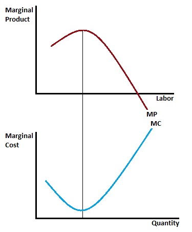
To further solidify this graphical understanding, the following video segment describes the curves as "mirror reflections" and breaks down the graph into stages corresponding to increasing and diminishing returns.

This direct link between the physical process of production (marginal product) and the financial costs (marginal cost) is a cornerstone of the theory of the firm, and we will build on it in future lessons.

Conclusion

In this lesson, we have forged the crucial link between production and costs. You now understand not only what the marginal cost curve looks like, but why it has its characteristic U-shape.

Here are your key takeaways:

• Inverse Relationship: The relationship between marginal product (MP) and marginal cost (MC) is inverse. When one is rising, the other is falling.
• The Cause: This relationship is driven by the law of diminishing marginal returns. Initially, specialization leads to increasing MP and falling MC. Eventually, fixed inputs become a constraint, causing diminishing MP and rising MC.
• The Formula: The relationship can be expressed by the formula $MC=\frac{w}{MP}$, where $w$ is the wage rate.
• Graphical Mirror: The MP and MC curves are graphical "mirror images." The maximum point of the MP curve corresponds to the minimum point of the MC curve.

We have now thoroughly covered the mechanics of a firm's costs in the short run. In our next lesson, we will shift our focus to the long run, where all inputs are variable. We will introduce the Long-Run Average Total Cost (LRATC) curve and explore the important concepts of economies and diseconomies of scale, which help explain the size and structure of firms in an industry.