Economies and Diseconomies of Scale

Introduction

Hello! Welcome back. In our last few lessons, we've taken a deep dive into the cost structure of a firm, but our focus has been exclusively on the short run—a period where at least one input, like the size of a factory, is fixed. This led us to understand concepts like diminishing marginal returns and the U-shaped marginal cost curve.

Today, we shift our perspective to the long run. In economics, the long run isn't a specific amount of time; it's a planning horizon where all inputs are variable. A firm can not only hire more workers but also build a bigger factory, invest in more machinery, or fundamentally change its scale of operation.

This lesson addresses the learning outcome: Describe economies and diseconomies of scale using the long-run average total cost curve. We will explore how a firm's average costs change as it scales up its production, a crucial factor in determining the size of firms and the structure of industries.

1. From Short-Run to Long-Run Costs

In the short run, a firm operates on a single Short-Run Average Total Cost (SRATC) curve, determined by its fixed level of capital (e.g., its factory size). In the long run, the firm can choose from many different factory sizes. Each potential size has its own SRATC curve.

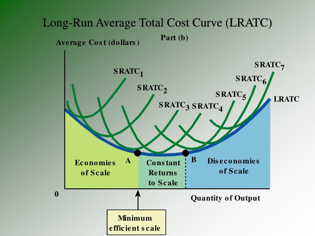
The Long-Run Average Total Cost (LRATC) curve represents the lowest possible average cost for producing any given level of output, as the firm has the flexibility to choose the optimal factory size for that output level. Therefore, the LRATC curve is the 'envelope' that contains all the possible SRATC curves.

To visualize this fundamental concept, please read the following section from the Lumen Learning textbook, which explains how the LRATC is constructed.

The concept of the LRATC as an "envelope curve" is one of the most important in this topic. The image below provides a clear illustration.

2. Economies of Scale: Getting Bigger Can Be Cheaper

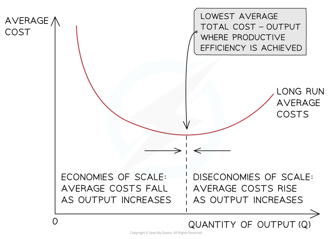
As you can see from the graph above, the LRATC curve initially slopes downward. This portion of the curve illustrates economies of scale, a situation where a firm's long-run average cost per unit of production decreases as its total output increases.

But why does this happen? The reasons are diverse and powerful. To understand the underlying causes of economies of scale, please watch the following video. It breaks down the reasons into two categories: those internal to the firm and those external to it.

The "technical" economies of scale mentioned in the video are particularly interesting. In many production processes, doubling the inputs can more than double the output. The Lumen Learning resource you looked at earlier provides an excellent example from the chemical industry, explaining that doubling the material cost of a pipe (related to its circumference) can increase its carrying capacity by a factor of four (related to its area). This is a great example of the physical and engineering realities that underpin economic principles.

3. Diseconomies of Scale: When Bigger is Not Better

If getting bigger were always better, we would expect to see industries dominated by single, colossal firms. This is often not the case because firms can also experience diseconomies of scale. This occurs when, beyond a certain point, a firm's long-run average cost per unit starts to increase as output rises. This is the upward-sloping portion of the U-shaped LRATC curve.

The reasons for diseconomies of scale are generally related to the challenges of managing an increasingly large and complex organization.

Let's return to the video from EconplusDal to understand these challenges.

As an IT analyst, you are likely familiar with how breakdowns in communication and coordination can create inefficiencies and raise costs in large projects or organizations. These are precisely the forces that drive diseconomies of scale.

4. Constant Returns to Scale and Minimum Efficient Scale

Between the regions of economies and diseconomies of scale lies a flat or nearly flat section on the LRATC curve. This area represents constant returns to scale, where expanding output does not significantly change the long-run average cost.

The point at which the LRATC curve reaches its lowest point is critically important. This is called the Minimum Efficient Scale (MES).

• Minimum Efficient Scale (MES): The lowest level of output at which a firm can minimize its long-run average costs.

It represents the scale of production where the firm has fully exploited all economies of scale, but has not yet begun to suffer from significant diseconomies of scale. The MES is crucial for understanding industry structure. For example, if the MES is very large relative to the size of the market, the industry might only be able to support a few large firms (or even just one, a natural monopoly).

For a precise definition of MES, please watch this short clip.

Conclusion

In this lesson, we made the important transition from short-run to long-run cost analysis. You learned how a firm's ability to change its scale of operation in the long run gives rise to a U-shaped long-run average total cost curve.

Here are your key takeaways:

• Long-Run Flexibility: In the long run, all inputs are variable, and the LRATC curve is the 'envelope' representing the minimum possible cost for any output level.
• Economies of Scale: The initial downward slope of the LRATC is caused by economies of scale, where larger size leads to lower average costs due to factors like specialization, bulk purchasing, and technical efficiencies.
• Diseconomies of Scale: The eventual upward slope of the LRATC is caused by diseconomies of scale, where excessive size leads to higher average costs due to management, communication, and coordination problems.
• Minimum Efficient Scale (MES): The point of lowest average cost on the LRATC curve. It is the most productively efficient scale for a firm to operate at.

We have now completed our module on the costs of production. You have a solid understanding of both short-run and long-run cost structures. In our next lesson, we will begin a new module by bringing revenue into the picture to understand how firms make decisions to maximize profit. Our first topic will be to distinguish between accounting profit and economic profit, a crucial first step in analyzing a firm's behavior.