Calculating and Graphing Per-Unit Costs

Introduction

Hello! In our last lesson, we focused on the "big picture" of a firm's costs, learning how to calculate and graph total fixed cost (TFC), total variable cost (TVC), and total cost (TC). We established that the shape of the total cost curves is a direct result of the law of diminishing marginal returns.

Today, we'll zoom in from the total to the per-unit level. While total costs are important, firms often make crucial decisions—like what price to charge or how much to produce—by thinking about costs on a per-unit basis. Our goal is to calculate and graph average fixed cost (AFC), average variable cost (AVC), average total cost (ATC), and marginal cost (MC). These four curves are among the most important tools in microeconomics, and mastering them is essential for understanding how firms behave.

1. Defining the Per-Unit Costs

Let's begin by defining our four new cost measures. They are all derived from the total cost concepts you learned in the previous lesson.

• Average Fixed Cost (AFC): The fixed cost per unit of output.
  $AFC=\frac{TFC}{Q}$
• Average Variable Cost (AVC): The variable cost per unit of output.
  $AVC=\frac{TVC}{Q}$
• Average Total Cost (ATC): The total cost per unit of output. It can be calculated in two ways:
  $ATC=\frac{TC}{Q}\text{or}ATC=AFC+AVC$
• Marginal Cost (MC): The additional cost of producing one more unit of output. Since fixed costs don't change with output, marginal cost is also the change in variable cost from one more unit.
  $MC=\frac{\Delta TC}{\Delta Q}=\frac{\Delta TVC}{\Delta Q}$
  (Where $\Delta$ means "change in").

These formulas are the building blocks for this lesson. You can find them neatly summarized in the resource below.

2. From Total Costs to Per-Unit Costs: A Worked Example

Now, let's see how to apply these formulas. The best way to understand the relationships is to work through an example, starting with the total costs and systematically calculating each per-unit cost.

The following video provides a detailed, step-by-step walkthrough of this process using a data table. As you watch, I encourage you to pause and try the calculations yourself to solidify your understanding.

3. Graphing the Per-Unit Cost Curves

With the calculations complete, we can now visualize these costs by plotting them on a graph. The shapes of these curves are not random; they reveal fundamental properties of a firm's production technology.

The next part of the video you just watched does exactly this, plotting the data from the table and explaining the economic intuition behind the shape of each curve.

After watching the video, let's summarize the key graphical relationships.

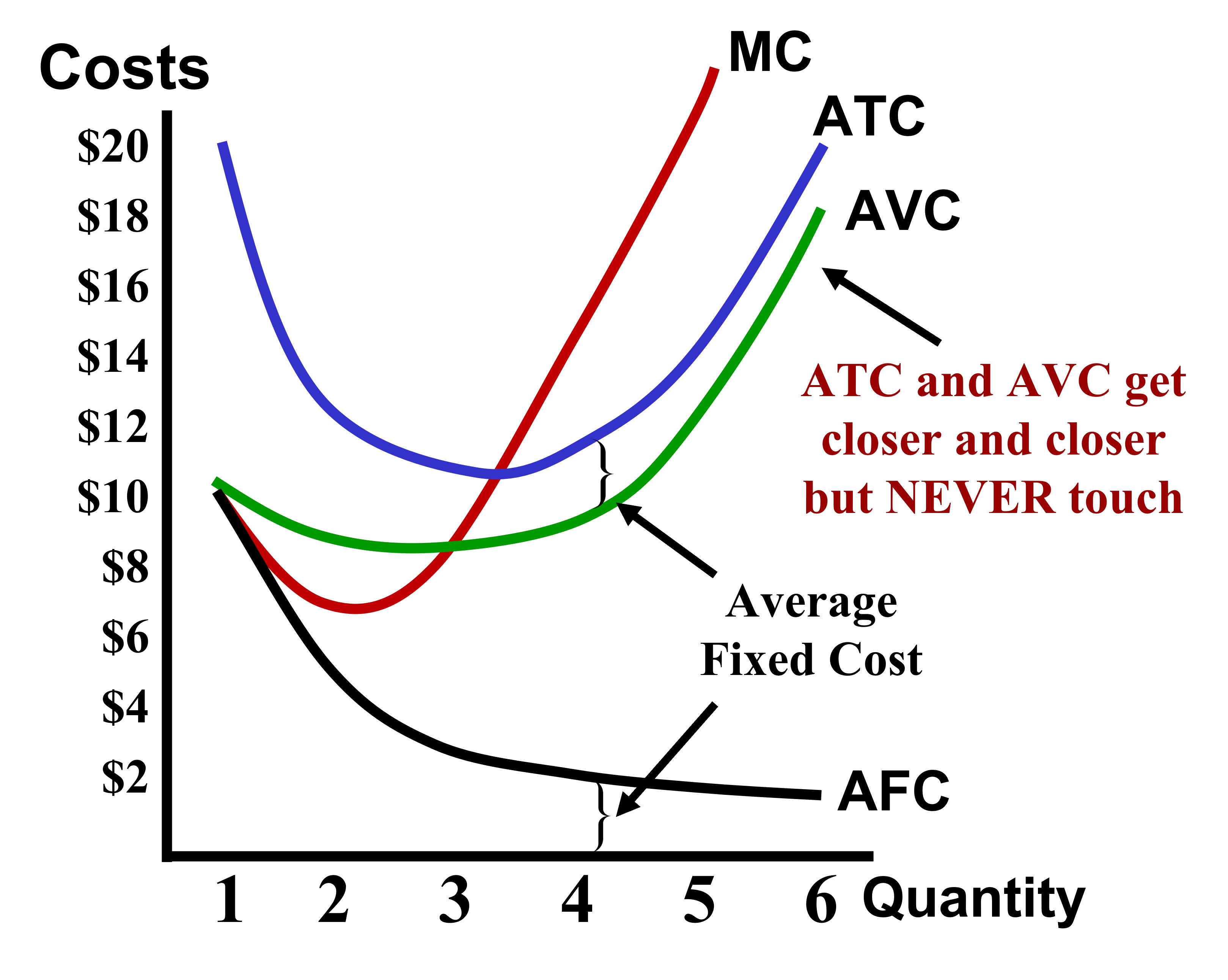
4. Reading and Applying the Cost Curve Graph

You can now calculate and graph the cost curves. The final step is to learn how to use these graphs to quickly find cost information and perform analysis.

The next video offers a concise summary of the graphical relationships and demonstrates a key practical skill: how to derive total cost figures directly from the per-unit cost graph. Given your technical background, you may find this geometric approach of identifying costs as areas on the graph particularly intuitive.

This skill of translating between per-unit costs and total costs using the graph is extremely useful and brings together the concepts from this lesson and the previous one.

Conclusion

In this lesson, you have learned to calculate and graph the four essential per-unit cost curves that are central to the theory of the firm. We've seen how these curves are derived from total costs and how their shapes reflect the underlying realities of production.

Here are your key takeaways:

• Four Key Definitions: You can now calculate AFC, AVC, ATC ($=\text{AFC}+\text{AVC}$), and MC.
• Characteristic Shapes: You can graph the always-falling AFC curve and the U-shaped AVC, ATC, and MC curves.
• The Crucial Intersection: The MC curve always intersects the AVC and ATC curves at their minimum points. This is because if the cost of the next unit (MC) is below the average, it pulls the average down. If it's above the average, it pulls the average up.
• Graphical Analysis: You can read a cost-curve graph to find a firm's per-unit and total costs at a specific level of output.

In the previous module, you learned about the marginal product of labor. In this lesson, you learned about marginal cost. Have you noticed that the marginal product curve was "hill-shaped" while the marginal cost curve is "U-shaped"? This is no coincidence. In our next lesson, we will formally connect these two concepts and explain why the relationship between the marginal cost curve and the marginal product curve is a mirror image, completing the link between production and cost.