Recommended resources
The freely available resources this lesson will direct you to.
Welcome back. In the previous lesson, ORDER BY inside OVER determined which products came first in a ranking. Now it will determine which period comes before or after another. You’ll use PostgreSQL’s LAG and LEAD functions to place neighboring sales values beside the current value, then calculate month-over-month changes.
This is a common analyst task, but the arithmetic is only trustworthy if each row represents the right period and the ordering matches the business question.
What counts as the previous row?
LAG(value) retrieves a value from an earlier row; LEAD(value) retrieves one from a later row. Both use the ordering specified inside OVER. For monthly revenue by region, the basic pattern is:
LAG(revenue) OVER (
    PARTITION BY region
    ORDER BY sales_month
)
This gives each region its own chronological sequence. On a February row, LAG can return January’s revenue for that region. Replacing LAG with LEAD would return March’s revenue. Neither function collapses rows: the current and neighboring values appear together on the February row.
Watch Data with Baraa’s SQL Value Window Functions for the mechanics. Focus on the relationship between the ordered rows and the values returned, rather than memorizing the video’s SQL dialect.
SQL Value Window Functions | LEAD, LAG, FIRST_VALUE, LAST_VALUE | #SQL Course 25
Data with Baraa’s SQL Value Window Functions shows how LAG and LEAD retrieve values at an offset from the current row.
Watch arguments and ordering for the expression, offset, and default arguments. Then watch neighboring values to see why the first row has no preceding value and the last has no following value. In PostgreSQL, an ORDER BY is essential for a meaningful chronological comparison, although the syntax does not require one.
Without an explicit offset, both functions move one row. At the beginning of a region’s sequence, LAG returns NULL by default; at the end, LEAD does. That NULL means no row exists at the requested position. It does not mean sales were zero.
Give each period one row
Before comparing months, decide the grain of the input. If an orders table contains many transactions per month, applying LAG(total_amount) directly would compare orders, not monthly totals. First aggregate to one row per region and month:
SELECT
    region,
    date_trunc('month', order_date)::date AS sales_month,
    SUM(total_amount) AS revenue
FROM orders
GROUP BY
    region,
    date_trunc('month', order_date)::date;
The year remains part of sales_month, so January in one year sorts after December in the preceding year. The resulting (region, sales_month) combination should identify one row. Duplicate rows for that combination would make “previous month’s revenue” ambiguous.
For a PostgreSQL example of this aggregate-then-compare pattern, read the LAG Analysis section of Crunchy Data’s Window Functions for Data Analysis with Postgres. It uses days rather than months, but the choice of grain works the same way.
Window Functions for Data Analysis with Postgres
Read Crunchy Data’s Window Functions for Data Analysis with Postgres to see a grouped sales result used as the input to LAG.
In the “LAG Analysis” section, start at the sentence about already having data grouped by day. Read the daily comparison through the sentence about LEAD, stopping before “Rolling averages.” Focus on why DailySales must be calculated before its rows can be compared.
We’ll use a small, already-aggregated table below so you can inspect every comparison. If you have a PostgreSQL session, you can run the SQL as you go.
CREATE TEMP TABLE monthly_sales (
    region text NOT NULL,
    sales_month date NOT NULL,
    revenue numeric(12, 2) NOT NULL,
    PRIMARY KEY (region, sales_month)
);

INSERT INTO monthly_sales (region, sales_month, revenue)
VALUES
    ('North', DATE '2025-01-01', 1000),
    ('North', DATE '2025-02-01', 1200),
    ('North', DATE '2025-03-01',  900),
    ('South', DATE '2025-01-01',  500),
    ('South', DATE '2025-02-01',    0),
    ('South', DATE '2025-03-01',  800);
Notice the distinction between South’s February revenue of zero, which is a recorded value, and a month with no row. That distinction will matter when interpreting a change.
Calculate backward and forward changes
Define the subtraction before writing it: change from the previous month is current revenue minus previous revenue. A positive result is an increase. For a percentage change, divide that difference by the previous revenue—not the current revenue—and multiply by 100.
The video’s month-over-month example demonstrates this calculation. Its MONTH(...) syntax is not the PostgreSQL monthly grouping used above, so use the PostgreSQL query that follows for implementation.
SQL Value Window Functions | LEAD, LAG, FIRST_VALUE, LAST_VALUE | #SQL Course 25
Return to SQL Value Window Functions for its month-over-month sales example.
Watch monthly change. Follow the progression from monthly totals to previous-month sales, absolute difference, and percentage difference. The video also shows why integer arithmetic can produce an unwanted zero when calculating a percentage; our PostgreSQL query uses numeric revenue and 100.0.
Here, a CTE makes the neighboring values available by name for the final calculations:
WITH adjacent_months AS (
    SELECT
        region,
        sales_month,
        revenue,
        LAG(revenue) OVER (
            PARTITION BY region
            ORDER BY sales_month
        ) AS previous_revenue,
        LEAD(revenue) OVER (
            PARTITION BY region
            ORDER BY sales_month
        ) AS next_revenue
    FROM monthly_sales
)
SELECT
    region,
    sales_month,
    revenue,
    previous_revenue,
    revenue - previous_revenue AS change_from_previous,
    ROUND(
        100.0 * (revenue - previous_revenue)
        / NULLIF(previous_revenue, 0),
        1
    ) AS pct_change_from_previous,
    next_revenue,
    next_revenue - revenue AS change_to_next
FROM adjacent_months
ORDER BY region, sales_month;
| region | sales_month | revenue | previous_revenue | change_from_previous | pct_change_from_previous | next_revenue | change_to_next |
|---|---|---|---|---|---|---|---|
| North | 2025-01-01 | 1000 | NULL | NULL | NULL | 1200 | 200 |
| North | 2025-02-01 | 1200 | 1000 | 200 | 20.0 | 900 | -300 |
| North | 2025-03-01 | 900 | 1200 | -300 | -25.0 | NULL | NULL |
| South | 2025-01-01 | 500 | NULL | NULL | NULL | 0 | -500 |
| South | 2025-02-01 | 0 | 500 | -500 | -100.0 | 800 | 800 |
| South | 2025-03-01 | 800 | 0 | 800 | NULL | NULL | NULL |
North’s February increase is 200, or 20% of January’s 1,000. On that same February row, LEAD shows that March’s revenue is 300 lower than February’s. The two change columns answer differently oriented questions: one looks back from the current period; the other looks ahead from it.
South’s March absolute increase is 800, but a conventional percentage change from a zero baseline is undefined. NULLIF(previous_revenue, 0) turns that denominator into NULL, so PostgreSQL returns NULL rather than raising a division-by-zero error. Do not report that result as 0%: “undefined from a zero baseline” is the more accurate interpretation. Similarly, the first month’s missing comparison remains NULL rather than becoming a fabricated zero-sales month.
Check what “one period earlier” really means
LAG and LEAD count rows, not calendar intervals. If North’s February row were missing, LAG(revenue) on North’s March row would retrieve January’s 1,000. Calling the resulting difference a month-over-month change would be misleading: those observations are two months apart.
If missing periods are possible, retrieve the neighboring date as well as its value and check it before labeling a change:
WITH available_months AS (
    SELECT *
    FROM monthly_sales
    WHERE NOT (
        region = 'North'
        AND sales_month = DATE '2025-02-01'
    )
),
paired_months AS (
    SELECT
        region,
        sales_month,
        revenue,
        LAG(sales_month) OVER (
            PARTITION BY region ORDER BY sales_month
        ) AS previous_month,
        LAG(revenue) OVER (
            PARTITION BY region ORDER BY sales_month
        ) AS previous_revenue
    FROM available_months
)
SELECT
    region,
    sales_month,
    previous_month,
    CASE
        WHEN previous_month =
             (sales_month - INTERVAL '1 month')::date
        THEN revenue - previous_revenue
    END AS month_over_month_change
FROM paired_months
WHERE region = 'North'
ORDER BY sales_month;
In this deliberately incomplete example, March’s previous_month is January, but month_over_month_change is NULL because January is not the preceding calendar month. The query does not invent a February value. Whether a real missing month should be filled with zero depends on what the absence of a row means in the source data.
Both functions can also take a larger offset: LAG(revenue, 2) looks back two rows, and LEAD(revenue, 2) looks forward two. The image below depicts a four-row offset in complete quarterly data. For example, the previous bonus beside 2018 quarter 1 comes from 2017 quarter 1.
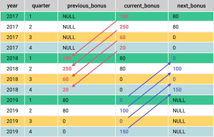
That four-row approach only represents the same quarter in another year if the quarterly sequence is complete and correctly ordered. Also notice that the image does not restart at each year: partitioning by year would prevent a comparison from reaching the preceding year. In your regional sales query, by contrast, partitioning by region prevents a value from one region being mistaken for another’s.
Key takeaways
LAG places a preceding row’s value beside the current row; LEAD places a following row’s value there. Aggregate to the intended time grain first, use PARTITION BY for independent groups, and order each group chronologically. Subtract in a stated direction, divide percentage change by the comparison period’s value, and preserve meaningful NULLs at boundaries or zero baselines. Most importantly, verify that an adjacent row is actually the adjacent period you intend to report.
Next lesson, you’ll keep the same ordered-window foundation but calculate across multiple rows at once, using window frames for running totals and moving averages.