Recommended resources
The freely available resources this lesson will direct you to.
- Running & Rolling Total | Moving & Rolling Average | SQL Key Data Analysis Conceptswww.youtube.com
- SQL Running Total | Advance SQL | Rolling N months SUM, AVG, MIN, MAXwww.youtube.com
- Running Totals and Moving Averages · YeSQLtheartofpostgresql.com
- Window Functions for Data Analysis with Postgreswww.crunchydata.com
Welcome back. In the previous lesson, you used LAG and LEAD to compare a month with a neighboring row. This time, each result will use several rows: all months so far for a running total, or a small group of recent months for a moving average.
These calculations are common in analyst reporting. A cumulative revenue chart shows progress over time; a moving average makes a noisy monthly trend easier to read. In both cases, the crucial question is: which rows contribute to the value shown for this month?
The frame inside a window
You already know that PARTITION BY region creates independent regional sequences and ORDER BY sales_month puts each sequence in time order. A window frame narrows that ordered sequence to the rows used for the calculation at the current row.
For example, ROWS BETWEEN 2 PRECEDING AND CURRENT ROW includes the current row and up to two rows before it. As the current row changes, that frame moves with it. At the beginning of a region, fewer than three rows may exist; PostgreSQL uses the rows that are available.

Watch Running & Rolling Total | Moving & Rolling Average from Data with Baraa for a visual comparison of a growing running total and a sliding calculation. Treat its frame descriptions as intuition rather than as a statement of PostgreSQL’s exact default frame, which we’ll clarify below.
Running & Rolling Total | Moving & Rolling Average | SQL Key Data Analysis Concepts
Data with Baraa’s video shows how changing the frame changes which values enter an aggregate.
Watch the distinction between running and rolling totals, then the running total. Continue through the sliding example, following which monthly values are included as the current month advances.
A frame does not remove rows from the result. Like LAG, a windowed SUM or AVG adds a calculated value beside each input row.
Running totals: a frame that grows
We’ll reuse the monthly_sales sample table from the previous lesson. It contains one row per (region, sales_month), including a recorded revenue of zero for South in February. If you opened a new PostgreSQL session, recreate that temporary table using the previous lesson’s setup before running these queries.
To show revenue accumulated through each month, start the frame at the beginning of the region and end it at the current row:
SELECT
    region,
    sales_month,
    revenue,
    SUM(revenue) OVER (
        PARTITION BY region
        ORDER BY sales_month
        ROWS BETWEEN UNBOUNDED PRECEDING AND CURRENT ROW
    ) AS running_revenue
FROM monthly_sales
ORDER BY region, sales_month;
| region | sales_month | revenue | running_revenue |
|---|---|---|---|
| North | 2025-01-01 | 1000 | 1000 |
| North | 2025-02-01 | 1200 | 2200 |
| North | 2025-03-01 | 900 | 3100 |
| South | 2025-01-01 | 500 | 500 |
| South | 2025-02-01 | 0 | 500 |
| South | 2025-03-01 | 800 | 1300 |
North’s March result is the sum of its January, February, and March revenue: 3,100. South begins its own running total at 500. Its February zero is included, but does not increase the total.
The two ORDER BY clauses have different jobs. The one inside OVER defines the order used for the calculation. The one at the end of the query arranges the displayed results. Without an ORDER BY inside OVER, SUM(revenue) OVER (PARTITION BY region) would show each region’s final total on every row, not a running total.
You may also see a running total written as SUM(revenue) OVER (PARTITION BY region ORDER BY sales_month). It produces the same figures here because each region has only one row per month. In PostgreSQL, however, an ordered window defaults to a RANGE frame through the current row, which includes other rows tied on the ordering value. The explicit ROWS frame above states precisely that we want to accumulate row by row.
Read Running Totals and Moving Averages from YeSQL to see that default, a sliding alternative, and the effect of ties in one short PostgreSQL treatment.
Running Totals and Moving Averages · YeSQL
YeSQL’s “Running Totals and Moving Averages” makes the contents of each frame visible with an accompanying array, so you can check what SUM or AVG actually receives.
After the opening generate_series(1, 5) query and its result table, read the growing frame. In “Moving averages: fix the frame width,” read the sliding example, including its SQL and results. Finally, in “ROWS vs RANGE,” read the peer comparison, including the query and result table; notice why a tied ordering value can make a RANGE total jump.
Moving averages: a frame that slides
A running total retains every earlier month. A three-row moving average instead uses the current month and the two preceding rows. When April arrives, for example, January drops out of April’s three-row frame; the calculation uses February, March, and April.
The next image illustrates a two-row version. Its first result uses only the current row because no earlier row exists; later results use the current and previous rows within the same home_type group.
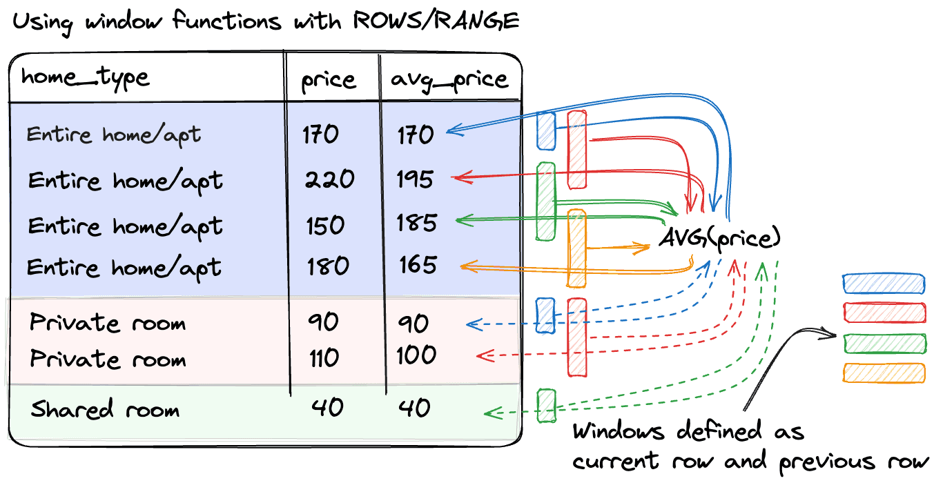
The video’s average examples also show why the direction of the frame matters. A frame using FOLLOWING brings future rows into today’s value; for a trend reported as of the current month, we usually want preceding rows instead.
Running & Rolling Total | Moving & Rolling Average | SQL Key Data Analysis Concepts
Return to Data with Baraa’s video for the average calculations. Compare its changing frames with the trailing frame we’ll use in PostgreSQL.
Watch the averages within partitions, then the custom frame. Notice that the latter example can include a following row; our query below deliberately looks backward.
Here is the trailing three-row average for the regional sales data. COUNT(*) uses the same named frame so the result also tells us how many rows contributed:
SELECT
    region,
    sales_month,
    revenue,
    COUNT(*) OVER trailing_three AS rows_in_frame,
    ROUND(
        AVG(revenue) OVER trailing_three,
        2
    ) AS moving_avg_3
FROM monthly_sales
WINDOW trailing_three AS (
    PARTITION BY region
    ORDER BY sales_month
    ROWS BETWEEN 2 PRECEDING AND CURRENT ROW
)
ORDER BY region, sales_month;
| region | sales_month | revenue | rows_in_frame | moving_avg_3 |
|---|---|---|---|---|
| North | 2025-01-01 | 1000 | 1 | 1000.00 |
| North | 2025-02-01 | 1200 | 2 | 1100.00 |
| North | 2025-03-01 | 900 | 3 | 1033.33 |
| South | 2025-01-01 | 500 | 1 | 500.00 |
| South | 2025-02-01 | 0 | 2 | 250.00 |
| South | 2025-03-01 | 800 | 3 | 433.33 |
North’s March average uses 1,000, 1,200, and 900. South’s March average uses 500, 0, and 800; a recorded zero counts as an observation. January’s and February’s averages use only one and two rows respectively, rather than dividing by three when three rows do not yet exist.
WINDOW trailing_three AS (...) simply gives the frame a name so that COUNT and AVG cannot accidentally use different definitions. You could write the same OVER (...) specification beside each function instead.
Decide what “three months” means
The SQL above specifies three rows, not necessarily three consecutive calendar months. This is the same distinction that mattered for LAG in the previous lesson. If South’s February row were absent, its March frame would include January and March, and the two-row average would not represent two consecutive months. If earlier months were available, a three-row frame could reach even further back to fill its three positions.
Before labeling a result “three-month moving average,” establish that the input has one row per region and month and that the relevant months are present. Whether a missing month should be represented by zero depends on the source data and the metric definition; a missing row is not automatically zero revenue.
Also decide how to report the start of a series. The query above reports an average of available rows, with rows_in_frame making the short frames visible. If a report requires three observed revenue values before displaying an average, you can use the named frame in this expression within the same SELECT:
CASE
    WHEN COUNT(revenue) OVER trailing_three = 3
    THEN ROUND(AVG(revenue) OVER trailing_three, 2)
END AS full_3_observation_avg
That would return NULL for January and February in each region. COUNT(revenue) checks for non-null revenue values; it still does not prove that those observations are consecutive calendar months. The appropriate choice—partial average or no result until the frame is complete—belongs in the metric definition.
Finally, keep the order unambiguous. The sample table has a unique month within each region, so ORDER BY sales_month is sufficient. If multiple input rows share an ordering value, ROWS counts their positions but needs an additional ordering key, such as a unique transaction ID, to make those positions deterministic. Better yet, for monthly revenue, aggregate transactions to one row per region and month before applying the frame.
Key takeaways
A running total uses a frame from the start of a partition through the current row. A moving average uses a frame that slides, such as ROWS BETWEEN 2 PRECEDING AND CURRENT ROW for up to three rows. PARTITION BY keeps regions independent, while the window’s ORDER BY determines what “preceding” means. Explicit frames, unique ordering, and a clear policy for missing or early periods make the resulting metric defensible.
Next lesson, you’ll combine intermediate query steps with window functions to build a fuller analytical query from raw data through reported metrics.