Parallel Scan: Foundations and Applications

Introduction

In our previous lesson, we explored the parallel reduction primitive, focusing on how a hierarchical, tree-based algorithm can be optimized to efficiently reduce a large array to a single value on a GPU. We saw that performance hinges on managing architectural details like warp divergence and shared memory bank conflicts.

This lesson builds directly on those concepts to tackle a related, but more general, data-parallel primitive. We will address the learning outcome: Describe the parallel scan (prefix sum) primitive and its application in data-parallel algorithms.

A scan, or prefix sum, takes an array of numbers and an associative operator (like addition) and returns an array of the same size. However, instead of just the final sum, it returns all the intermediate "running totals." This primitive is a fundamental building block for a surprisingly wide range of parallel algorithms that seem inherently sequential, such as stream filtering, sorting, and certain kinds of graph and tree operations.

We will examine the core challenge in parallelizing scan, explore classic algorithms that solve it, and see how it is used to enable other complex data-parallel tasks.

1. Defining Scan (Prefix Sum)

A scan operation takes an input array $[a_0,a_1,\dots ,a_{n-1}]$ and a binary associative operator $\oplus$. There are two main variants:

• Inclusive Scan: The output element at index $i$ is the reduction of all input elements up to and including $a_i$.
  ${\text{out}}_i=a_0\oplus a_1\oplus \cdots \oplus a_i$
• Exclusive Scan: The output element at index $i$ is the reduction of all input elements before $a_i$. The first element is the identity value $I$ for the operator $\oplus$.
  ${\text{out}}_i=a_0\oplus a_1\oplus \cdots \oplus a_{i-1}$

For example, for the input [3 1 7 4] with the + operator (identity 0):

• Inclusive scan: [3, 4, 11, 15]
• Exclusive scan: [0, 3, 4, 11]

The two forms are easily convertible, so we will often just refer to "scan."

A sequential implementation is straightforward, but it contains a critical data dependency: out[i] = out[i-1] + in[i]. This dependency makes a direct parallelization impossible, as each output depends on the previously computed one. We need a different approach.

2. Parallel Scan Algorithms

As with reduction, the key to an efficient parallel scan is a tree-based approach. We will look at two main algorithms that represent a classic trade-off between simplicity and efficiency.

Algorithm 1: A Simple but Work-Inefficient Approach (Hillis & Steele)

The first parallel algorithm we'll consider is intuitive. It works in logarithmic steps. In each step d, every element k adds the value from an element 2^(d-1) positions away.

This is exactly the algorithm described in the next segment of the video. It's simple to understand but has a significant drawback.

This algorithm achieves logarithmic time complexity, which is a massive improvement over the linear time of the sequential version. However, its work complexity of $O(n\log n)$ means it performs much more total work than the optimal $O(n)$. For large arrays, this extra factor of $\log n$ is very costly.

Algorithm 2: A Work-Efficient Approach (Blelloch Scan)

A more advanced algorithm, proposed by Guy Blelloch, achieves both logarithmic time and linear work, making it asymptotically optimal. It consists of two passes over the data, which can be visualized as traversing up and down a binary tree.

1. Reduce (Up-Sweep) Phase: In this phase, we traverse from the leaves of the tree towards the root. Each parent node in the tree stores the sum of its children's values. This is essentially a parallel reduction, where we store all the intermediate partial sums along the way. At the end of this phase, the root node (the last element of the array) contains the sum of the entire array.

2. Down-Sweep Phase: We traverse from the root back to the leaves. Starting by setting the root's value to the identity (0 for addition), we use the partial sums computed during the up-sweep to calculate the final prefix sums. At each node, we pass its current value to its left child. For the right child, we pass the sum of the parent's current value and the stored partial sum of the left child (from the up-sweep).

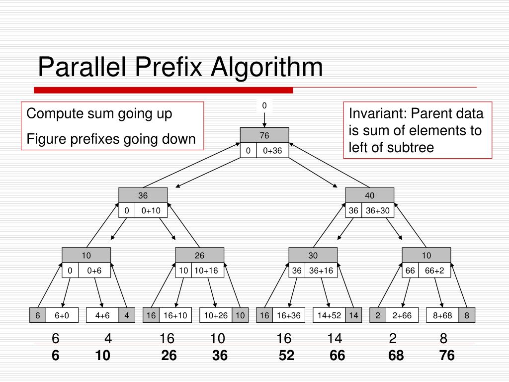
This two-pass method is more complex to reason about, but its work efficiency makes it the foundation of most high-performance scan implementations.

The GPU Gems chapter on scan provides pseudocode for these two phases, which helps formalize the process shown in the video.

3. Implementation on a GPU: A Hierarchical Approach

Just like with parallel reduction, implementing scan on a GPU involves a hierarchical strategy that maps the algorithm to the GPU's architecture of warps, blocks, and grids.

• Intra-Warp Scan: For the 32 threads within a warp, a simple O(w log w) Hillis-Steele style scan is often used. Because all threads in a warp execute in lockstep (SIMT), the work-inefficiency is less of a concern than the algorithmic simplicity and lack of synchronization overhead.

• Intra-Block Scan: To scan across a thread block, we compose the results of intra-warp scans. Each warp computes its own scan. Then, the partial sum from each warp is collected, and a single warp scans these partial sums. Finally, these results are broadcast back to the other warps, which add the block-level prefix to their local results. This is a direct application of the "divide and conquer" strategy.

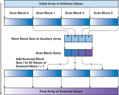
• Grid-Level Scan (Large Arrays): To handle arrays larger than a single block can process, we use multiple kernel launches, just as we did for reduction.

  1. Divide the input array into chunks, one per block.
  2. Kernel 1: Each block scans its local chunk and writes the block's total sum to an auxiliary array.
  3. Kernel 2: A second kernel (often just one block) is launched to scan the auxiliary array of block sums.
  4. Kernel 3: A final kernel adds the scanned block sums to the corresponding chunks from the first step.

This multi-pass process is visualized effectively in the following image.

The design of these hierarchical algorithms is a deep topic. For a more detailed perspective on how they are constructed, the following technical report is an excellent resource, though not required reading.

4. Applications of Parallel Scan

The true power of scan lies in its ability to convert seemingly sequential problems into parallel ones. By pre-calculating prefix sums, we can determine the output position of elements in parallel, eliminating data dependencies.

Stream Compaction (Filtering)

A canonical example is stream compaction. The goal is to take an input array and a predicate (a true/false condition) and produce a new array containing only the elements for which the predicate is true, in their original order.

A sequential approach would loop through the array, check the predicate, and copy the element to an output array using a counter. This is sequential because the output position of element i depends on how many preceding elements passed the predicate.

Scan solves this elegantly:

1. Create a flag array: Generate a binary array where 1 represents an element that passes the predicate and 0 represents one that fails.
2. Scan the flag array: Perform an exclusive scan on the flag array. The result for each element is the count of all preceding 1s. This resulting value is precisely the destination index in the compacted output array!
3. Scatter: In parallel, each thread i checks if its element passed the predicate. If it did, it uses the index from the scanned flag array to write (scatter) its value to the correct position in the output array.

Other important applications of scan include:

• Radix Sort: Scan is used within each step of a parallel radix sort to determine the new positions of elements based on their current bit values.
• Summed-Area Tables: Used in image processing for fast box blurs, this is computed by performing a scan on all rows, followed by a scan on all columns.
• Polynomial Evaluation: Scan can be used to evaluate polynomials in parallel.

Conclusion

In this lesson, we demystified the parallel scan primitive, a cornerstone of data-parallel programming. While its implementation is more intricate than that of reduction, the underlying principles are similar, relying on tree-based algorithms and a hierarchical mapping to the GPU architecture.

Key Takeaways:

• Scan (Prefix Sum) is a primitive that computes the "running total" for an array, producing an output array of intermediate reductions.
• Simple sequential implementations have strong data dependencies, making them unsuitable for parallel execution.
• Work-efficient parallel scan algorithms like the Blelloch scan use a two-pass up-sweep (reduce) and down-sweep approach to achieve $O(n)$ work and $O(\log n)$ time.
• Efficient GPU implementations use a hierarchical strategy (intra-warp, intra-block, grid-level) and require multiple kernel launches to process large arrays.
• Scan is a powerful building block for other algorithms, most notably stream compaction, where it is used to calculate output addresses in parallel, breaking sequential dependencies.

Preview of the Next Lesson:

We have now covered two fundamental data-parallel primitives: reduction and scan. In the next lesson, we will shift our focus to a workload that is at the heart of nearly all modern deep learning: matrix multiplication (GEMM). We will see how this operation is parallelized on GPUs using a technique called tiling, which leverages shared memory to manage data reuse and maximize computational throughput.