Optimizing CUDA Occupancy and Performance

Introduction

Welcome to the final lesson of this module. In our previous lessons, we've explored fundamental parallel primitives like reduction and scan, and you've seen how their efficient implementation requires careful mapping to the GPU's hierarchical architecture. We've laid the groundwork for writing correct parallel code. Now, we shift our focus to making it fast.

This lesson addresses the learning outcome: Analyze how thread block size and grid dimensions can be tuned to maximize occupancy and performance.

We will delve into one of the most critical aspects of GPU performance tuning: launch configuration. You'll learn why GPUs rely on massive multithreading to achieve high performance, a concept known as latency hiding. We will then define occupancy as a key metric for this capability and analyze the hardware resources that constrain it. Finally, we'll explore the trade-offs involved in choosing the right block and grid sizes and, crucially, understand when maximizing occupancy leads to better performance and when it doesn't.

This knowledge is essential for bridging the gap between using high-level AI frameworks and understanding how to design and optimize the underlying systems for peak efficiency.

1. The Core Challenge: Hiding Latency

The fundamental reason GPUs are designed for massive parallelism is not just to divide work, but to hide latency. Latency is the delay between requesting data and receiving it. Accessing data from the main GPU memory (global memory) is incredibly slow compared to the speed of the arithmetic logic units (ALUs). A typical global memory access can take hundreds of clock cycles.

If a thread has to wait for data, the processing units on the GPU would sit idle, wasting enormous computational potential. The GPU's solution is to oversubscribe the hardware with threads. Threads are grouped into warps (typically 32 threads) for execution. When one warp stalls (e.g., waiting for a memory read), the SM's warp scheduler instantly switches to another resident warp that is ready to execute.

This process, known as latency hiding, ensures the execution units are always busy with useful work. However, this mechanism is only effective if there are enough resident warps on the SM to switch between. This is why simply launching 32 or 64 threads is insufficient; we need to launch thousands or tens of thousands to provide the scheduler with enough options.

The following video provides an excellent and detailed visualization of this process.

2. Occupancy: A Metric for Latency-Hiding Potential

We need a way to measure a kernel's potential for latency hiding. This metric is called occupancy.

Occupancy is the ratio of active warps on a Streaming Multiprocessor (SM) to the maximum number of warps that the SM can support. For example, if an SM can support a maximum of 64 warps and your kernel configuration allows 32 warps to be active, your occupancy is 50%.

A higher occupancy generally means the SM has more warps to choose from, improving its ability to hide latency. However, as we'll see, the relationship between occupancy and final performance is not always linear.

What determines how many warps can be active? The resources on an SM are finite. A thread block is only scheduled onto an SM if there are sufficient resources for all threads within that block. The primary limited resources per SM are:

• Registers: A large, fast register file is available to all threads on the SM. Each thread in your kernel uses a certain number of registers, determined by the compiler.
• Shared Memory: A fast, on-chip memory space that can be shared by all threads within a block.
• Thread/Warp Capacity: The SM has a hard limit on the total number of resident threads and warps it can handle simultaneously (e.g., 2048 threads or 64 warps on a Volta V100).
• Block Capacity: The SM also has a limit on the number of concurrent thread blocks it can manage.

The number of blocks that can run on an SM is limited by the most constrained of these resources. It's like a multi-dimensional game of Tetris, where you try to pack as many blocks as possible into the SM's finite resource pool.

3. Tuning Grid and Block Dimensions

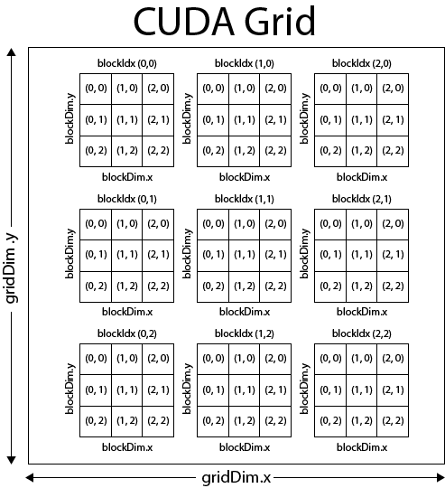
Now, let's connect this back to your kernel launch, which in CUDA C++ looks like kernel_name<<<grid_dim, block_dim, ...>>>. Understanding how to set grid_dim and block_dim is the key to controlling occupancy and performance.

Tuning Grid Dimensions (grid_dim)

The grid_dim parameter specifies the total number of thread blocks to launch. The goal here is simple: launch enough blocks to keep all SMs on the GPU busy.

• Guideline: The number of blocks in your grid should be significantly larger than the number of SMs on your GPU. A common practice is to aim for a multiple (e.g., 2x to 4x) of the number of SMs.
• Reasoning: This "oversubscription" ensures that as blocks complete their work and free up SM resources, the GPU's global scheduler has a ready supply of new blocks to dispatch. This prevents SMs from going idle and maximizes overall device utilization. In most cases, you'll set the grid size based on your total data size, for example (num_elements + threads_per_block - 1) / threads_per_block.

Tuning Block Dimensions (block_dim)

The block_dim parameter, specifying the number of threads per block, is where the more complex tuning happens. This choice directly impacts the resource consumption of each block.

• Guideline 1: Block size should be a multiple of the warp size (32).

  • Reasoning: The SM issues instructions to full warps. If your block size is not a multiple of 32 (e.g., 100 threads), the last warp will contain only 4 active threads (100 % 32 = 4). The SM still allocates resources and issues instructions for all 32 lanes, but 28 of them will be masked off and do no useful work. This wastes execution resources.

• Guideline 2: Choose a block size that balances parallelism and resource usage.

  • Commonly effective block sizes are 128, 256, and 512.
  • Too small (e.g., 32 or 64): A block with only one or two warps has limited ability to hide latency within its own instruction stream. You might also need an extremely large number of small blocks to achieve high occupancy, which can introduce scheduling overhead.
  • Too large (e.g., 1024): A large block might consume too many registers or too much shared memory. For example, if a thread needs 64 registers, a block of 1024 threads would require 65,536 registers. If your SM's register file is that size, only one such block can be resident on the SM, severely limiting your occupancy.

The trade-off is clear: you want blocks large enough to expose parallelism, but not so large that their resource footprint prevents multiple blocks from co-residing on an SM.

Calculating Theoretical Occupancy

You can predict a kernel's maximum possible occupancy without even running it. The theoretical occupancy is determined by the most limiting resource.

For a given GPU architecture and kernel:

1. Blocks per SM (Register Limit): floor(Total_Registers_per_SM / (Registers_per_Thread * Threads_per_Block))
2. Blocks per SM (Shared Memory Limit): floor(Total_Shared_Memory_per_SM / Shared_Memory_per_Block)
3. Blocks per SM (Warp/Thread Limit): floor(Max_Threads_per_SM / Threads_per_Block)

The actual number of blocks that can fit is min() of these values (and the architectural max blocks per SM). The theoretical occupancy is then:

$$\text{Occupancy}=\frac{(\text{Actual Blocks per SM}\times \text{Threads per Block})}{\text{Max Threads per SM}}$$

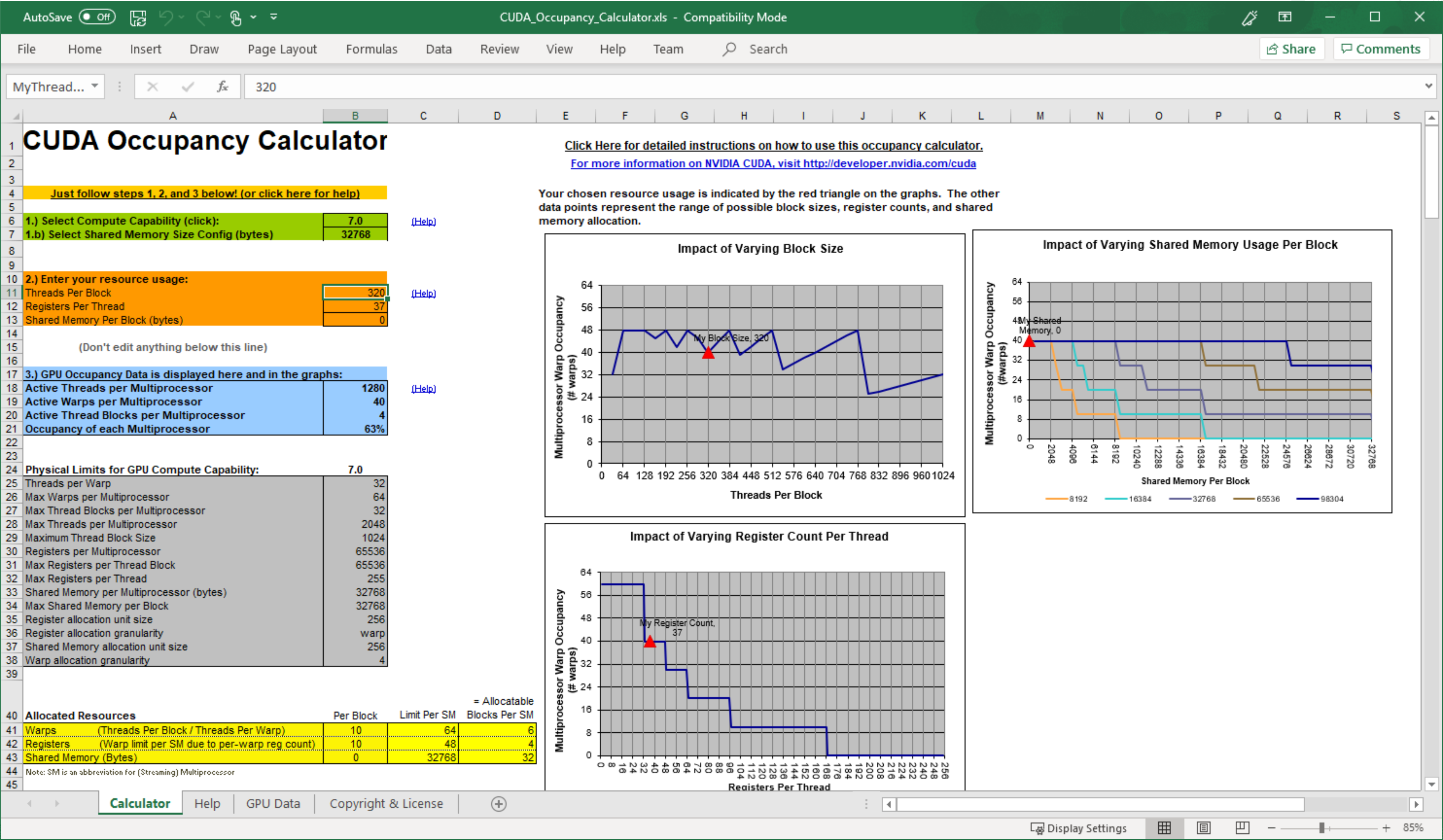
To make this analysis easier, NVIDIA provides a tool.

4. The Critical Caveat: Occupancy Is Not the Goal

Maximizing occupancy is a common starting point for optimization, but it is not the ultimate goal. The goal is to maximize performance, which means minimizing runtime. Sometimes, a configuration with lower occupancy can result in higher performance.

This paradox arises when occupancy is not the primary performance bottleneck. Kernels are often limited by one of two things:

• Compute-Bound: The runtime is limited by the speed of arithmetic calculations.
• Memory-Bound: The runtime is limited by the bandwidth of the memory system.

For a memory-bound kernel, once you achieve sufficient occupancy (often as low as 25-50%) to hide the memory access latency, adding more warps doesn't help. All those additional warps just end up waiting in line to access the same, saturated memory bus. In this scenario, other factors like memory coalescing (which we'll cover later) are far more important.

Conversely, a kernel with higher register usage per thread might have lower occupancy but could perform better if those extra registers are used to avoid costly re-computations or spills to slow local memory.

The puzzle demonstrates that a systematic approach is required. Don't just chase 100% occupancy. Instead, use profiling tools to identify the true bottleneck and focus your optimization efforts there.

Conclusion

In this lesson, we moved from writing correct parallel code to analyzing what makes it performant. You've learned how to reason about the fundamental trade-offs in GPU kernel launch configurations.

Key Takeaways:

• GPUs use massive multithreading to hide memory latency, which is the primary source of stalls.
• Occupancy measures the number of active warps on an SM and is a proxy for latency-hiding capability.
• Occupancy is limited by per-SM resources: registers, shared memory, and thread/block capacity.
• Grid dimensions should be large enough to saturate all SMs on the device.
• Thread block size is a critical tuning parameter. It must be a multiple of 32 and is typically best in the 128-512 range, balancing parallelism with resource consumption.
• Occupancy is a means, not the goal. Once sufficient occupancy is achieved to hide latency, performance is often limited by other factors, such as memory bandwidth. Analyzing the true bottleneck is key.

Preview of the Next Lesson:

With this foundation in performance tuning, you are now ready to tackle one of the most important workloads in deep learning. In the next lesson, we will begin a new module, "Parallelizing Machine Learning Workloads," by answering the question: How is matrix multiplication parallelized on GPUs using tiling and shared memory? You will see a direct application of today's concepts, as choosing the right tile and block size is a classic occupancy optimization problem.