Parallel Reduction: Concepts and GPU Implementation

Introduction

Welcome back! In our last lesson, we established the critical role of shared memory and synchronization primitives like __syncthreads(). We saw that to achieve high performance, you must consciously manage data movement to exploit the fast, on-chip scratchpad memory, and carefully coordinate threads to avoid race conditions and performance pitfalls like bank conflicts.

This lesson puts that theory into practice. We will tackle the learning outcome: Describe the parallel reduction primitive and a common GPU implementation pattern.

A reduction is an operation that collapses a collection of elements into a single result using a binary operator. Operations like summing a vector, finding its maximum element, or calculating its L2-norm are all reductions. They are ubiquitous in machine learning, from normalizing probabilities in a softmax function to calculating loss values.

We will embark on a step-by-step journey to develop an efficient parallel reduction algorithm on the GPU. Starting with a simple but flawed idea, we will progressively refine it, applying the principles of shared memory, synchronization, and conflict avoidance you've just learned. This process is a case study in GPU optimization and will equip you with a powerful, reusable algorithmic pattern.

1. What is a Reduction?

Formally, a reduction applies an associative binary operator to an input sequence, reducing it to a single value. For an operator $\oplus$ and an input sequence $[x_0,x_1,...,x_{N-1}]$, the reduction is $x_0\oplus x_1\oplus ...\oplus x_{N-1}$.

Common examples include:

• Sum: Operator is +, identity is 0.
• Product: Operator is *, identity is 1.
• Max/Min: Operator is max()/min(), identity is $-\infty$/$+\infty$.

To understand why this primitive is so important in AI systems, let's watch a short introduction.

A serial implementation is trivial: you initialize an accumulator and loop through the elements. However, our goal is to leverage massive parallelism. A simple loop is inherently sequential and won't do.

2. The Core Idea: A Tree-Based Parallel Algorithm

The standard parallel approach to reduction is to structure the computation as a binary tree. At each level of the tree, we perform pairwise operations, halving the number of elements to be processed in the next level. This continues until only one element remains.

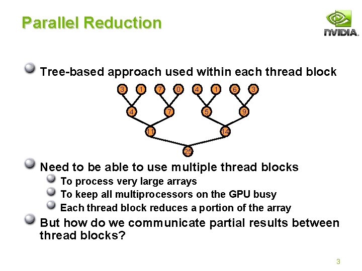
This tree-based method is a classic "divide and conquer" strategy. Each thread block on the GPU will be responsible for reducing a portion of the input array using this pattern. The core of our implementation will be realizing this tree structure efficiently using shared memory and threads.

3. A Step-by-Step GPU Implementation

Let's build a common and highly optimized GPU reduction kernel. We'll start with a naive implementation and iteratively fix its performance problems. This journey reveals key GPU optimization principles.

The seminal guide for this process is NVIDIA's paper on the topic. While the specific performance numbers are from an older architecture, the architectural principles and optimization steps remain fundamental.

Step 1: Naive Approach and Warp Divergence

Our first instinct might be to implement the reduction tree directly. We load data into shared memory and then, in a loop, have threads pair up to add values. A common first attempt looks like this (pseudo-code):

// Inside a kernel, after loading data into sdata[]
for (unsigned int s = 1; s < blockDim.x; s *= 2) {
    __syncthreads();
    if (threadIdx.x % (2 * s) == 0) {
        sdata[threadIdx.x] += sdata[threadIdx.x + s];
    }
}

In this "interleaved addressing" pattern, thread i adds the value from thread i+s. The if condition ensures only the even-numbered threads in each pair are active.

The Problem: This pattern suffers from massive warp divergence. In the first iteration, half the threads in a warp are inactive. In the second, three-quarters are inactive, and so on. Since a warp executes a single instruction for all its threads, the active threads are forced to wait for the inactive ones, leading to extremely poor hardware utilization. The modulo operator (%) is also computationally expensive.

This is "Kernel 1" in the Optimizing Parallel Reduction in CUDA PDF (slide 9).

Step 2: Fixing Divergence and Hitting Bank Conflicts

We can improve on this by rearranging the thread mapping to keep active threads contiguous.

// A better, but still flawed, approach
for (unsigned int s = blockDim.x / 2; s > 0; s >>= 1) {
    __syncthreads();
    if (threadIdx.x < s) {
        sdata[threadIdx.x] += sdata[threadIdx.x + s];
    }
}

Here, we reverse the loop. In each step, the first s threads are active. This is much better for divergence, as entire warps are active in early stages, and only the "boundary" warp might be partially active.

The New Problem: As you'll recall from our last lesson, this introduces shared memory bank conflicts. The video below explains exactly why this access pattern (sdata[tid] and sdata[tid + s]) is problematic.

The key insight is that when the stride s is a multiple of the number of banks (32), threadIdx.x and threadIdx.x + s will often map to the same bank for different threads in a warp, causing serialization.

Step 3: The Conflict-Free Implementation Pattern

The solution demonstrated in the video you just watched is the core of the common GPU implementation pattern. By using a decreasing stride and having the first s threads perform the additions, we ensure that the threads accessing shared memory are contiguous. This results in sequential, conflict-free access to the shared memory banks.

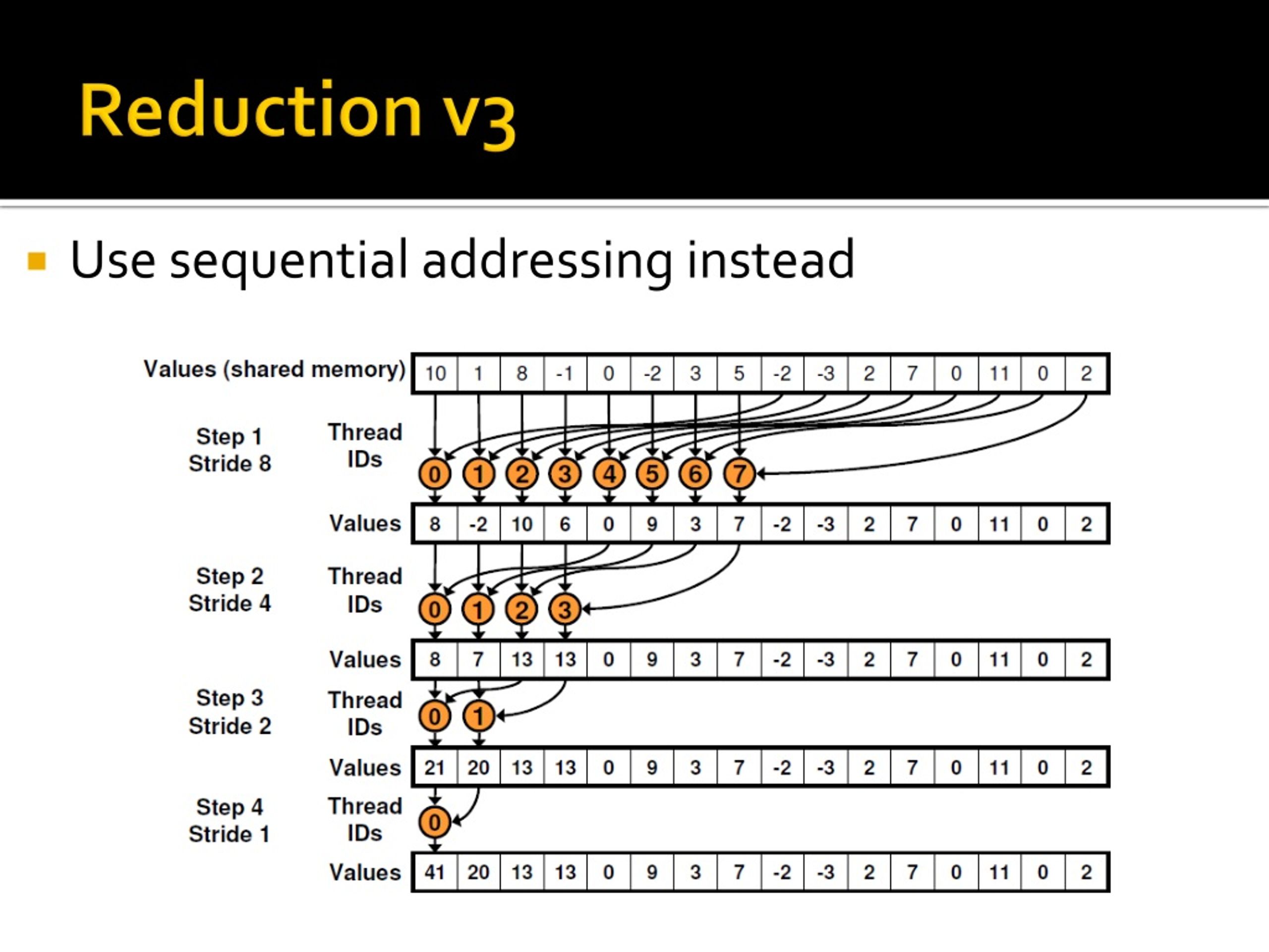
This pattern, which corresponds to "Kernel 3" in the NVIDIA PDF, successfully implements a correct and reasonably efficient reduction within a single thread block.

4. Advanced Optimizations for High Performance

A correct algorithm is just the starting point. To approach the peak memory bandwidth of the GPU (which is the goal for a memory-bound algorithm like reduction), we need further optimizations.

Optimization 1: More Work Per Thread (Thread Coarsening)

In the previous pattern, if a block has 256 threads, half of them are idle in the very first step of the shared memory reduction. We can do better.

The idea is to have each thread process multiple elements from global memory sequentially before the cooperative shared memory reduction begins. Each thread computes a partial sum in its own private register, and only then do the threads cooperate to sum up these partials.

This technique is sometimes called thread coarsening or register blocking.

This strategy has two major benefits:

1. It increases the work-to-overhead ratio, improving the arithmetic intensity of the kernel.
2. It reduces the total number of global memory transactions if the access pattern is coalesced.

This corresponds to "Kernel 7" in the NVIDIA PDF and the concept of "register blocking" in the Modern GPU resource.

Optimization 2: Handling Large Inputs (Multi-Block Reduction)

Our pattern works well within a single block, but a block has a limited size (e.g., 1024 threads) and a finite amount of shared memory. To reduce an array of millions of elements, we need a strategy to combine results between blocks.

Since there's no cheap, global __syncthreads() across all blocks of a grid, the standard solution is to use multiple kernel launches:

1. Kernel 1: Launch a grid of many blocks. Each block reduces a large chunk of the input (using the optimized pattern from above) and writes its single partial result to a temporary array in global memory.
2. Kernel 2: Launch a single block (or a small number of blocks) to reduce the partial results from Kernel 1.
3. This can be repeated recursively, but in practice two launches are usually sufficient.

A kernel launch acts as an implicit global synchronization point.

Optimization 3: Reducing Instruction Overhead (Loop Unrolling & Warp Shuffles)

The for loop for the shared memory reduction still incurs instruction overhead (branching, counter updates). For the final stages of the reduction, when the number of active threads (s) is less than or equal to the warp size (32), all active threads are in the same warp.

Since threads in a warp execute in lockstep, we can unroll these last loop iterations. This eliminates the loop overhead and, critically, removes the need for __syncthreads() between these steps, as warp-synchronous execution is guaranteed.

On modern GPUs, this is taken a step further with warp-level primitives like __shfl_down_sync(). These instructions allow threads within a warp to exchange data directly through registers, completely bypassing shared memory for an even faster intra-warp reduction.

The general, modern hierarchical pattern is:

1. Thread-level: Each thread reduces many elements from global memory into a register.
2. Warp-level: The threads in each warp reduce their partial sums using shuffle instructions.
3. Block-level: The single result from each warp is written to shared memory, and a single warp performs a final reduction on these results.
4. Grid-level: Results from each block are combined using a second kernel launch or atomics.

5. Reductions in Practice: Frameworks like PyTorch

Given your background, it's insightful to see how these low-level concepts manifest in high-level frameworks. When you call torch.sum(), PyTorch's backend dispatcher selects or generates a highly optimized kernel that uses these very techniques. For smaller inputs, it might dispatch a single-block kernel; for larger ones, a multi-block kernel. Through code generation systems like Triton, it can even create specialized reduction kernels on the fly, tuned for the specific data type and size of your tensor, often employing the full hierarchical strategy we've outlined.

Conclusion

In this lesson, we dissected the parallel reduction primitive and constructed a common, highly-optimized GPU implementation pattern. We saw how building performant kernels is an iterative process of identifying and eliminating bottlenecks, from architectural hazards like warp divergence and bank conflicts to instruction and memory overhead.

Key Takeaways:

• Parallel reduction is a fundamental data-parallel primitive that uses a tree-based algorithm to compute a single result in logarithmic time.
• A common GPU implementation involves a hierarchical strategy: sequential reduction within threads (thread coarsening), cooperative reduction within warps (shuffles), cooperative reduction within a block (shared memory), and finally, reduction across blocks (multiple kernel launches or atomics).
• Optimizing reduction is a case study in applying core GPU principles: maximizing parallelism, avoiding warp divergence, ensuring memory coalescing, eliminating bank conflicts, and reducing instruction overhead through loop unrolling.

Preview of the Next Lesson:

The reduction algorithm is closely related to another essential primitive: the parallel scan (or prefix sum). A scan operation also processes an array but produces an array of intermediate results, where each output element is the reduction of all input elements up to that point. In the next lesson, we will see how the patterns and techniques we developed for reduction can be adapted to build an efficient parallel scan algorithm.