Verifying Machine Learning Computations with Vector and Matrix Dimensions

Hello. In the previous lesson, you learned to select statistical tests based on the structure of a model comparison: pairing, independent units, metric type, and training variation. We now shift from statistical validity to a similarly practical form of validation: checking whether an ML expression can exist at all.

Dimension checking is an interview skill and an engineering debugging habit. A shape mismatch in a feature pipeline, layer boundary, loss function, or gradient update often reveals a mistaken assumption about what an axis represents. By the end of this lesson, you should be able to annotate common ML computations with vector and matrix dimensions, identify invalid products or additions, and explain the result shape of valid operations.

---

Dimensions are a contract

A vector in ${\mathbb{R}}^d$ contains $d$ numbers. When we need to be explicit about orientation, we write it as a column vector:

$$x\in {\mathbb{R}}^{d\times 1}$$

A matrix $A\in {\mathbb{R}}^{m\times n}$ has $m$ rows and $n$ columns:

$$A\in {\mathbb{R}}^{m\times n}$$

The notation is not mere bookkeeping. It states what information an array holds and which operations make sense. In ML, dimensions usually correspond to meaningful axes:

Symbol	Typical interpretation
$N$	number of examples in a batch or dataset
$d$	input-feature dimension
$h$	hidden-layer width
$K$	number of output classes
$V$	vocabulary size
$D$	embedding dimension

For example, a tabular batch with $N$ examples and $d$ features per example is conventionally represented as:

$$X\in {\mathbb{R}}^{N\times d}$$

Each row is one example; each column is one feature. If a batch has 64 examples with 1280 features each, then:

$$X\in {\mathbb{R}}^{64\times 1280}$$

This row-per-example convention is common in NumPy, pandas-derived ML pipelines, and PyTorch batch-first tensors. Some mathematical texts instead arrange examples as columns. Either convention is valid, but silently mixing them is not.

A useful habit is to state your convention before manipulating an expression:

“I will use rows for examples, so $X$ has shape $N\times d$.”

That sentence prevents many interview and implementation errors.

---

The one multiplication rule to apply mechanically

For matrix multiplication, the inner dimensions must match:

$$A\in {\mathbb{R}}^{m\times n},B\in {\mathbb{R}}^{n\times p}$$

Then the product exists and has the outer dimensions:

$$AB\in {\mathbb{R}}^{m\times p}$$

A compact way to reason about it is:

$$(m\times \cancel{n})(\cancel{n}\times p)=m\times p$$

The matching $n$ dimensions are consumed by the dot products. The remaining outer dimensions describe the result.

For example:

$$W\in {\mathbb{R}}^{10\times 3072},x\in {\mathbb{R}}^{3072\times 1}$$

Therefore:

$$Wx\in {\mathbb{R}}^{10\times 1}$$

This is the shape of a linear classifier that receives a flattened CIFAR-like image with 3072 pixel-channel values and emits ten class scores.

Matrix multiplication is not element-wise multiplication

If $A$ and $B$ both have shape $m\times n$, then element-wise multiplication is valid:

$$A\odot B\in {\mathbb{R}}^{m\times n}$$

Each entry is multiplied with the entry in the same position. This is different from $AB$, which may be undefined even though $A$ and $B$ have identical shapes.

For instance, if:

$$A,B\in {\mathbb{R}}^{64\times 1280}$$

then $A\odot B$ is valid and has shape $64\times 1280$. But $AB$ is invalid because the inner dimensions would be $1280$ and $64$, which do not match.

This distinction is especially relevant in deep-learning code, where * may mean element-wise multiplication while a dedicated operator or function performs matrix multiplication.

---

Vectors, transposes, and the two products people confuse

A vector is often written without an explicit orientation:

$$x\in {\mathbb{R}}^d$$

For dimensional reasoning, make the orientation visible. Let:

$$x\in {\mathbb{R}}^{d\times 1},y\in {\mathbb{R}}^{d\times 1}$$

Then two apparently similar expressions have very different meanings.

Inner product: a scalar

$$x^{T}y$$

has shape:

$$(1\times d)(d\times 1)=1\times 1$$

So $x^{T}y$ is a scalar. It measures an alignment or weighted sum. Linear regression scores, cosine similarity numerators, and neuron pre-activations use this kind of operation.

Outer product: a matrix

$$x{y}^T$$

has shape:

$$(d\times 1)(1\times d)=d\times d$$

So $x{y}^T$ is a matrix. Outer products appear in covariance estimates, low-rank updates, and gradient formulas.

For $d=512$, an inner product produces one number, while an outer product produces a $512\times 512$ matrix containing 262,144 values. If you expected a score but obtained a large square matrix, an accidental transpose is a likely cause.

The transpose reverses dimensions:

$$A\in {\mathbb{R}}^{m\times n}$$ $$A^T\in {\mathbb{R}}^{n\times m}$$

It also reverses the order of a product:

$$(AB{)}^T=B^T{A}^T$$

That reversal matters. Matrix multiplication is generally not commutative:

$$AB\ne BA$$

Often, one order is valid while the other is not.

---

Linear regression: a complete shape audit

Suppose a regression model predicts one scalar value per example. Under the row-per-example convention:

$$X\in {\mathbb{R}}^{N\times d}$$ $$w\in {\mathbb{R}}^{d\times 1}$$ $$b\in \mathbb{R}$$

The prediction equation is:

$$\hat{y}=Xw+b$$

Check it in stages:

$$Xw\in {\mathbb{R}}^{N\times 1}$$

Adding scalar $b$ to every predicted value preserves the shape:

$$\hat{y}\in {\mathbb{R}}^{N\times 1}$$

The target vector must therefore be shaped compatibly:

$$y\in {\mathbb{R}}^{N\times 1}$$

A common squared-error objective is:

$$L(w)=\frac{1}{N}{\Vert Xw+b-y\Vert }_2^2$$

The residual vector has shape:

$$Xw+b-y\in {\mathbb{R}}^{N\times 1}$$

The norm reduces this vector to a scalar:

$$L(w)\in \mathbb{R}$$

This is an important semantic checkpoint: a training loss must normally be scalar after its reduction across examples and output dimensions.

The gradient with respect to the weight vector has the same shape as the weight vector:

$${\nabla }_{w}L\in {\mathbb{R}}^{d\times 1}$$

For squared error, a common form is:

$${\nabla }_{w}L=\frac{2}{N}{X}^T(Xw+b-y)$$

The dimensions verify the result:

$$X^T\in {\mathbb{R}}^{d\times N}$$ $$Xw+b-y\in {\mathbb{R}}^{N\times 1}$$ $$X^T(Xw+b-y)\in {\mathbb{R}}^{d\times 1}$$

That must be true: gradient descent needs to subtract an update from $w$, so the update and $w$ must have identical shapes.

$$w\leftarrow w-\eta {\nabla }_{w}L$$

Here, $\eta$ is a scalar learning rate.

---

Fully connected neural-network layers

A dense layer maps $d$ input features to $h$ hidden features. Under a column-vector convention for a single example:

$$x\in {\mathbb{R}}^{d\times 1}$$ $$W\in {\mathbb{R}}^{h\times d}$$ $$b\in {\mathbb{R}}^{h\times 1}$$

The layer computation is:

$$z=Wx+b$$ $$a=\varphi (z)$$

where $\varphi$ is an element-wise activation function such as ReLU.

The shape audit is:

$$Wx\in {\mathbb{R}}^{h\times 1}$$ $$z\in {\mathbb{R}}^{h\times 1}$$ $$a\in {\mathbb{R}}^{h\times 1}$$

The rule behind the weight shape is simple:

A dense layer weight matrix has one row per output unit and one column per input feature.

If a layer maps 1280 input features to 256 hidden features:

$$W_1\in {\mathbb{R}}^{256\times 1280}$$

A classifier head that maps 256 hidden features to $K=8$ classes has:

$$W_2\in {\mathbb{R}}^{8\times 256}$$

For one example:

$$x\in {\mathbb{R}}^{1280\times 1}$$ $$h=\varphi (W_{1}x+b_1)\in {\mathbb{R}}^{256\times 1}$$ $$z=W_{2}h+b_2\in {\mathbb{R}}^{8\times 1}$$

The resulting vector $z$ contains eight logits, one per class.

Batched dense layers and framework conventions

For an entire batch, place examples in rows:

$$X\in {\mathbb{R}}^{N\times d}$$

The same layer can be written as:

$$Z=X{W}^T+1b^T$$

where:

$$W\in {\mathbb{R}}^{h\times d}$$ $$b\in {\mathbb{R}}^{h\times 1}$$ $$Z\in {\mathbb{R}}^{N\times h}$$

The product checks out:

$$X{W}^T\in {\mathbb{R}}^{N\times d}{\mathbb{R}}^{d\times h}={\mathbb{R}}^{N\times h}$$

Framework APIs often hide some of this. For example, a dense-layer module may store weights as $(h,d)$, while accepting batched input shaped $(N,d)$. Internally, it effectively uses the transposed weight orientation necessary for the batched product. When debugging, check both the documented weight layout and the documented input layout.

---

Addition is stricter than multiplication—except when broadcasting is intentional

Ordinary matrix addition requires identical shapes:

$$A+B\text{is valid only if}\mathrm{shape}(A)=\mathrm{shape}(B)$$

Thus:

$$A\in {\mathbb{R}}^{N\times h},B\in {\mathbb{R}}^{N\times h}$$

can be added, while an $N\times h$ matrix cannot ordinarily be added to an $N\times d$ matrix when $h\ne d$.

ML libraries add an important practical extension: broadcasting. A smaller array can be treated as if it were repeated along an axis when the dimensions are compatible.

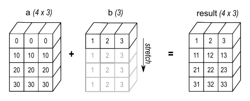
For a batched dense layer, the pre-activation output has shape:

$$X{W}^T\in {\mathbb{R}}^{N\times h}$$

The bias may be stored as a one-dimensional vector:

$$b\in {\mathbb{R}}^h$$

When adding $b$ to the batch, libraries such as NumPy and PyTorch align it with the final axis and apply the same bias to every example:

$$X{W}^T+b\in {\mathbb{R}}^{N\times h}$$

Conceptually, $b$ is repeated for each row. Efficient implementations generally do not materialize $N$ physical copies.

A broadcasting rule worth memorizing

Starting from the last axis, two dimensions are broadcast-compatible if they are:

• equal; or
• one of them is $1$; or
• one array has no corresponding leading dimension.

Examples:

Shapes	Valid?	Result shape	Typical ML interpretation
$(N,h)+(h)$	Yes	$(N,h)$	Add one bias vector to each example
$(N,h)+(1,h)$	Yes	$(N,h)$	Explicit row-shaped bias
$(N,h)+(N,1)$	Yes	$(N,h)$	Apply one scalar offset per example
$(N,h)+(N)$	Usually no	—	Ambiguous intended axis; reshape first
$(N,h)+(d)$	Only if $d=h$	$(N,h)$	Feature-wise addition

The suspicious case is especially common. If you have one scalar per example:

$$s\in {\mathbb{R}}^N$$

and want to add it to every hidden unit of the corresponding example, reshape it as:

$$s\in {\mathbb{R}}^{N\times 1}$$

before combining it with an $N\times h$ tensor. The extra dimension makes your intent explicit.

---

Common ML shape patterns

The following patterns recur in ML interviews, design discussions, and framework error messages.

Computation	Operand shapes	Result shape
Linear regression predictions	$X:N\times d,w:d\times 1$	$N\times 1$
Dense layer, batched examples	$X:N\times d,W^T:d\times h$	$N\times h$
Multiclass logits	$H:N\times h,W_{\text{out}}^T:h\times K$	$N\times K$
One-hot labels	$Y:N\times K$	$N\times K$
Per-example class label IDs	$y:N$	$N$
Feature covariance	$X_c^T:d\times N,X_c:N\times d$	$d\times d$
Example similarity matrix	$X:N\times d,X^T:d\times N$	$N\times N$
Embedding lookup	token IDs: $N\times T$, table: $V\times D$	$N\times T\times D$
Gradient of scalar loss with respect to $W$	$W:h\times d$	$h\times d$

Two lines in that table are easy to confuse:

$$X^{T}X\in {\mathbb{R}}^{d\times d}$$

is a feature-feature matrix, such as a covariance-related quantity, while:

$$X{X}^T\in {\mathbb{R}}^{N\times N}$$

compares examples with examples. Both may be dimensionally valid, but they answer different questions. Shape checking tells you whether code can run; axis meaning tells you whether it solves the intended problem.

---

A realistic debugging walkthrough

Suppose a perception feature service produces one 1280-dimensional vector per image, and an MLP classifier processes batches of 32 images.

The batch is:

$$X\in {\mathbb{R}}^{32\times 1280}$$

The first layer has 256 hidden units:

$$W_1\in {\mathbb{R}}^{256\times 1280}$$ $$b_1\in {\mathbb{R}}^{256}$$

The correct batch calculation is:

$$H=\varphi (X{W}_1^T+b_1)$$

Check each component:

$$X{W}_1^T\in {\mathbb{R}}^{32\times 1280}{\mathbb{R}}^{1280\times 256}={\mathbb{R}}^{32\times 256}$$

The bias broadcasts across the batch:

$${\mathbb{R}}^{32\times 256}+{\mathbb{R}}^{256}={\mathbb{R}}^{32\times 256}$$

Now assume the head predicts eight categories:

$$W_2\in {\mathbb{R}}^{8\times 256}$$ $$b_2\in {\mathbb{R}}^8$$

Then:

$$Z=H{W}_2^T+b_2$$

has shape:

$${\mathbb{R}}^{32\times 256}{\mathbb{R}}^{256\times 8}={\mathbb{R}}^{32\times 8}$$

Each row has eight logits for one image.

Now consider a plausible but wrong implementation:

$$H=X{W}_1+b_1$$

This attempts:

$${\mathbb{R}}^{32\times 1280}{\mathbb{R}}^{256\times 1280}$$

The inner dimensions are $1280$ and $256$, so the product is invalid. The repair is not to reshape arbitrarily. It is to determine the intended input and output axes, then use:

$$W_1^T\in {\mathbb{R}}^{1280\times 256}$$

An arbitrary reshape can silence an error while scrambling the meaning of features. A transpose is justified only when it restores the intended mathematical orientation.

---

An interview-ready dimension-checking method

When an interviewer gives you an equation, narrate your check rather than just declaring it valid or invalid.

1. Name each axis.
   “$N$ is batch size, $d$ is input dimension, and $h$ is hidden width.”

2. Write a shape beside every operand.
   For example:

   $$X:N\times d,W:h\times d,b:h$$

3. Check every multiplication locally.
   For $X{W}^T$, verify:

   $$(N\times d)(d\times h)=N\times h$$

4. Check every addition separately.
   “The bias is length $h$, so it broadcasts across the $N$ rows.”

5. Verify that the final shape matches the semantic goal.
   “A classifier with $K$ classes should emit $N\times K$ logits for a batch.”

A concise answer might sound like this:

“With examples as rows, $X$ is $N\times d$. A dense layer from $d$ inputs to $h$ outputs stores weights as $h\times d$, so the batch computation is $X{W}^T+b$, giving $N\times h$. The bias has one value per output unit and broadcasts over the batch. If the final layer has $K$ units, the logits are $N\times K$, which aligns with one label or one one-hot target vector per example.”

---

Key takeaways

Dimensions express the contract of an ML computation: what each axis represents, what operations are valid, and what the result means.

For matrix multiplication:

$$(m\times n)(n\times p)=m\times p$$

The inner dimensions must match, and the outer dimensions form the result. Addition generally requires identical shapes, though broadcasting can intentionally repeat a smaller array such as a bias across a batch.

For standard row-batched ML data:

$$X\in {\mathbb{R}}^{N\times d}$$

A dense layer mapping $d$ inputs to $h$ outputs commonly computes:

$$X{W}^T+b\in {\mathbb{R}}^{N\times h}$$

Finally, a valid shape is necessary but not sufficient. Both $X^{T}X$ and $X{X}^T$ may be valid, yet one represents feature relationships and the other example relationships. Always check both the algebra and the meaning of each axis.

Next, you will build on this notation to explain eigenvalues, eigenvectors, and singular value decomposition as tools for dimensionality reduction.