Comparing Model Variants with Statistical Hypothesis Testing

Hello. In the previous lesson, you learned to quantify uncertainty in a model metric and, crucially, to bootstrap the paired difference between two models evaluated on the same examples. Hypothesis tests use the same pairing principle but answer a narrower question: is the observed difference sufficiently incompatible with a specified no-difference assumption?

For ML interviews and release reviews, the important skill is not memorizing one formula. It is identifying what is being compared: two frozen models on one test set, two training procedures across resampled datasets, or two randomized production variants. By the end of this lesson, you should be able to select an appropriate test, state its null hypothesis and assumptions, interpret its p-value without overclaiming, and combine statistical evidence with practical and safety criteria.

---

The logic of a model-comparison test

A statistical hypothesis test begins with a deliberately skeptical baseline, the null hypothesis $H_0$. For two model variants, it often states that their relevant population performances are equal. The alternative hypothesis $H_1$ states the kind of difference you are looking for.

For a two-sided comparison of metric difference

$$\Delta =m_A-m_B,$$

the hypotheses are commonly:

$$H_0:\Delta =0$$ $$H_1:\Delta \ne 0$$

You choose a significance threshold, usually

$$\alpha =0.05,$$

before inspecting the final result. Under a valid test, $\alpha$ controls the long-run probability of a Type I error: rejecting $H_0$ when the null is actually true.

A p-value is:

Assuming the null hypothesis and the test’s assumptions are true, the probability of observing a result at least as incompatible with $H_0$ as the one obtained.

It is not:

• the probability that $H_0$ is true;
• the probability that the result occurred “by chance”;
• the size or importance of the model improvement;
• a launch recommendation.

The conventional decision rule is simple:

Result	Correct frequentist statement
$p<\alpha$	Reject $H_0$; the data provide evidence against the stated no-difference null.
$p\ge \alpha$	Fail to reject $H_0$; the data do not provide sufficient evidence against it at the chosen threshold.

“Fail to reject” is intentionally weaker than “the models are equal.” A small evaluation set, highly variable metric, or weak effect may all yield a non-significant result even when a meaningful difference exists. This is a Type II error risk; statistical power is the probability that a test detects a real effect of a specified size.

A useful interview-level distinction is:

• Statistical significance: is the result distinguishable from zero under the model and assumptions?
• Practical significance: is the plausible improvement large enough to matter for cost, quality, latency, safety, or another release criterion?

For a pedestrian detector, a 0.1 percentage-point aggregate improvement might be statistically significant on millions of frames yet irrelevant—or unacceptable if it coincides with worse recall for pedestrians at night.

---

First choose the comparison target

The phrase “compare two models” hides several different statistical questions. Selecting a test begins by naming the target.

What you are comparing	Typical data structure	Appropriate approach
Two fixed binary classifiers evaluated on the same held-out examples	Paired correct/incorrect outcomes	McNemar test
Two fixed models with a complex metric such as mAP, AUROC, F1, or calibration error	Paired predictions on the same evaluation units	Paired bootstrap interval; paired permutation test when a formal test is required
Two training procedures whose performance varies across dataset splits	Paired scores across repeated resampling	A variance-corrected repeated-CV test or 5x2 cross-validation test
Two randomized online variants	Independent randomized units, often users	Experiment-specific test or regression at the randomization unit
Several fixed classifiers on the same examples	Paired binary correctness for more than two models	Omnibus test such as Cochran’s Q, then corrected pairwise tests

The most common interview mistake is to take $k$ cross-validation scores from Model A and Model B and run an ordinary paired $t$-test as if the folds were independent. They are not: their training sets overlap heavily, so the score differences are correlated. Ignoring that correlation underestimates uncertainty and produces too many false positives.

Before proceeding, study the two main settings: paired fixed-model comparison and resampling-based algorithm comparison.

---

McNemar’s test: two fixed classifiers, one shared test set

Suppose two frozen classifier versions have been run on exactly the same labeled test examples. Each example yields a pair of binary outcomes: whether Model 1 was correct and whether Model 2 was correct.

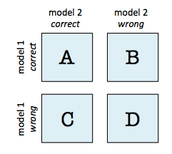
Let the cells mean:

	Model 2 correct	Model 2 wrong
Model 1 correct	$A$	$B$
Model 1 wrong	$C$	$D$

The two accuracies are:

$${\mathrm{Acc}}_1=\frac{A+B}{A+B+C+D}$$ $${\mathrm{Acc}}_2=\frac{A+C}{A+B+C+D}$$

At first glance, all four cells appear relevant. For McNemar’s test, however, the evidence lies in the discordant pairs:

• $B$: Model 1 correct and Model 2 wrong;
• $C$: Model 1 wrong and Model 2 correct.

Cells $A$ and $D$ are agreements. They help describe overall performance, but they do not indicate which model wins where they disagree.

McNemar’s null hypothesis is:

$$H_0:p_B=p_C$$

Under $H_0$, among cases where one model succeeds and the other fails, each model is equally likely to be the one that succeeds. The two-sided alternative is:

$$H_1:p_B\ne p_C$$

For a sufficiently large number of discordant pairs, the continuity-corrected McNemar statistic is:

$${\chi }^2=\frac{{\left(\left|B-C\right|-1\right)}^2}{B+C}$$

Under the null, this is approximately distributed as chi-squared with one degree of freedom. Software converts the statistic into a p-value. When the total number of discordant pairs $B+C$ is small, use the exact binomial version rather than relying on the chi-squared approximation.

Worked example

Consider two pedestrian-classification models evaluated on $1000$ independent, representative driving scenarios:

	Candidate correct	Candidate wrong
Baseline correct	$A=900$	$B=33$
Baseline wrong	$C=12$	$D=55$

The baseline accuracy is:

$${\mathrm{Acc}}_{\text{baseline}}=\frac{900+33}{1000}=0.933$$

The candidate accuracy is:

$${\mathrm{Acc}}_{\text{candidate}}=\frac{900+12}{1000}=0.912$$

Here, Model 1 is the baseline. It is correct when the candidate is wrong on 33 examples, while the candidate is correct when the baseline is wrong on only 12 examples. The observed accuracy difference is $2.1$ percentage points in favor of the baseline.

The continuity-corrected statistic is:

$${\chi }^2=\frac{(|33-12|-1{)}^2}{33+12}=\frac{400}{45}\approx 8.89$$

This corresponds to approximately:

$$p\approx 0.003$$

At a pre-specified $5\%$ threshold, reject the equal-performance null. A careful interpretation is:

On this defined evaluation population, the paired correctness outcomes provide evidence that the baseline and candidate have different accuracy. The observed difference favors the baseline by 2.1 percentage points.

Avoid adding claims the test did not establish. This result does not prove that the baseline will always outperform the candidate, that it is safer in every operating condition, or that its improvement is operationally important. You would still inspect scenario slices such as nighttime crossings, occluded pedestrians, and adverse weather.

Assumptions and limits

McNemar is an excellent answer when the interview prompt specifies two frozen classifiers evaluated once on the same labeled test set. But name its limitations:

1. Paired observations: both models must be evaluated on each same example.
2. Appropriate independent unit: driving frames from the same trip are not independent evidence. If trips are the meaningful independent unit, use a cluster-aware evaluation and resampling plan rather than treating every frame as unrelated.
3. Binary correctness: McNemar tests an accuracy-like correctness outcome. It does not directly compare mAP, AUROC, expected calibration error, or a latency-quality trade-off.
4. No training variance: it addresses uncertainty from the evaluation examples for these specific trained models, not seed-to-seed or training-data instability.

---

Complex metrics and unstable training procedures

For object detection, a release decision may center on mAP, recall at a safety-relevant operating point, or false negatives per scenario. Such metrics are not simple per-example Bernoulli outcomes. In this setting, the paired bootstrap method from the previous lesson is often more transparent:

1. Keep each model’s prediction paired with the same evaluation unit.
2. Resample those units—or trips, users, or scenes—with replacement.
3. Recompute both metrics and their difference for every replicate.
4. Construct a confidence interval for the paired difference.
5. Use the interval together with a pre-specified practical threshold.

If a binary reject/fail-to-reject decision is explicitly required for a complex metric, a paired permutation test can be suitable. Under the no-difference null, interchange the two models’ paired predictions within each unit, recompute the metric difference many times, and compare the observed difference against that null distribution. Preserve clusters during this process when the units are correlated.

The statistical question changes when the variants are not two frozen artifacts but two training procedures. For example:

• Procedure A uses a new augmentation policy.
• Procedure B uses the current augmentation policy.
• Each is retrained across multiple train/test splits.

Now training-set variation is part of what you need to measure. Ordinary $k$-fold scores are correlated because folds share much of their training data. A repeated-CV comparison therefore needs a variance correction, such as the Nadeau–Bengio corrected paired $t$-test; the 5x2 cross-validated paired $t$-test is another established choice for comparing two algorithms.

A strong concise answer to a cross-validation interview prompt is:

“Because scores from cross-validation folds are correlated through overlapping training sets, I would not use a naive paired $t$-test on fold scores. If my target is the expected performance difference between training procedures, I would use a repeated-CV comparison with an appropriate variance correction, such as Nadeau–Bengio, or a 5x2cv test. I would then retrain the selected pipeline and report final performance once on an untouched test set.”

That final untouched test set matters. Repeatedly tuning against the same “test” data turns it into a validation set and makes the final performance claim optimistic.

---

Interpretation: statistical evidence is not a release decision

A test should not be the sole gate for shipping a model. A production decision should combine:

• the metric difference and its uncertainty interval;
• a minimum practical effect threshold;
• scenario and demographic slices;
• guardrails, including latency, calibration, resource cost, and regressions;
• the representativeness of the evaluation data;
• the consequence of each error type.

Suppose an offline test reports:

$${\Delta }_{\text{pedestrian recall}}=0.014$$ $$p=0.02$$

The result is statistically significant at $5\%$, but it is incomplete. A disciplined follow-up asks:

• Was the test and primary metric selected before checking results?
• Is 1.4 percentage points greater than the operational threshold?
• Does the paired confidence interval support a practically meaningful gain?
• Did nighttime or rain slices regress?
• Is the test set route-disjoint and representative of deployment?
• Does the candidate increase latency beyond its service-level objective?

Conversely, if $p=0.12$, do not say “the models are the same.” Say:

“This evaluation did not provide enough evidence to reject the specified no-difference null at the chosen threshold. I would examine the confidence interval and power: the data may still be compatible with an improvement or regression large enough to matter.”

To demonstrate equivalence, define an acceptable margin in advance, such as an absolute recall difference no worse than $0.5$ percentage points, and use an equivalence-oriented procedure. Absence of significance is not evidence of equivalence.

One-sided versus two-sided tests

A one-sided alternative could be:

$$H_1:\Delta >0$$

Use it only when the direction was pre-specified and a harmful effect in the other direction would not be ignored. In safety-relevant ML, a two-sided assessment plus explicit guardrails is usually more defensible: a candidate that unexpectedly degrades performance must remain visible.

Many variants create a multiple-testing problem

If you compare 20 prompt variants, architectures, thresholds, or scenario slices at $5\%$, false positives become likely. This is especially relevant when a team searches across many experiments and celebrates the first small p-value.

Good practice is to:

• pre-specify a primary comparison and decision metric;
• treat exploratory results as exploratory;
• use an omnibus test before many pairwise comparisons when appropriate;
• adjust pairwise p-values, for example with Bonferroni when strong false-positive control is needed;
• confirm the selected candidate on fresh, untouched data.

For three or more fixed classifiers evaluated on the same labeled examples, Cochran’s Q is a paired omnibus test. If it finds evidence that at least one differs, follow with corrected pairwise tests rather than running every pair uncritically.

---

An interview-ready selection script

When asked how you would compare model variants, use this sequence:

1. Define the estimand and unit.
   “Am I comparing these two fitted model artifacts on the deployment population, or comparing two training procedures over plausible training sets? Is the independent unit a request, user, trip, clip, or frame?”

2. Confirm pairing and metric.
   “Were both variants evaluated on the same examples? Is the outcome binary correctness, an average loss, or a structured metric such as mAP?”

3. Select a test consistent with that structure.
   “For two fixed classifiers on one shared test set and a binary correct/incorrect outcome, I would use exact or asymptotic McNemar depending on the discordant count. For a structured metric, I would use paired cluster bootstrap uncertainty and, if needed, a paired permutation test. For retrained procedures across cross-validation splits, I would use a variance-corrected resampling comparison rather than a naive fold-level $t$-test.”

4. State the hypotheses and threshold before results.
   “My null is no difference in the stated target metric. I would usually use a two-sided test and pre-specify $\alpha$, power, and a minimum practically meaningful effect.”

5. Interpret without overclaiming.
   “A small p-value is evidence against the null under the assumptions, not a probability that the candidate is better. I would report the effect size, paired confidence interval, test population, and safety or business slices.”

---

Key takeaways

Hypothesis testing compares observed evidence with a stated null model. A p-value is the probability of results at least as extreme as those observed assuming the null is true; it is not the probability that the null is true. Rejecting a null supports evidence of a difference, while failing to reject does not establish equality.

For two fixed binary classifiers evaluated on the same held-out examples, McNemar’s test is the central method. Build the paired correctness table and focus on its discordant counts $B$ and $C$. Use its exact version when discordant data are limited, and do not apply it blindly to correlated video frames or non-binary metrics.

For structured metrics, preserve pairing through a paired, cluster-aware bootstrap and consider a paired permutation test when a formal hypothesis test is needed. For comparisons of training procedures across resampled splits, use a method that accounts for correlated folds, such as a corrected repeated-CV test or 5x2cv—not a naive $t$-test over folds.

Next, you will shift from statistical comparison to a complementary interview skill: checking whether common ML computations are dimensionally valid using vectors and matrices.