Dimensionality Reduction with Eigenvalues, Eigenvectors, and SVD

Hello. In the previous lesson, you treated dimensions as a contract: a matrix expression must be both shape-valid and semantically meaningful. That same discipline now makes PCA much easier to reason about. With examples as rows, we will move from a centered data matrix $X_c\in {\mathbb{R}}^{N\times d}$ to a lower-dimensional representation $Z\in {\mathbb{R}}^{N\times k}$, where $k<d$.

This lesson explains the linear-algebra story behind dimensionality reduction: eigenvectors identify useful directions, eigenvalues quantify variance along those directions, and singular value decomposition computes the same PCA structure directly from the data matrix. By the end, you should be able to give a concise, technically sound PCA explanation in an ML interview and describe the trade-offs that matter in a production or vision setting.

---

Eigenvectors: directions a transformation preserves

Before using eigenvectors for data, separate the general concept from PCA.

For a square matrix $A$, a nonzero vector $v$ is an eigenvector if applying $A$ changes only its scale, not its direction:

$$Av=\lambda v$$

The scalar $\lambda$ is the associated eigenvalue. If $\lambda =3$, the vector is stretched threefold. If $\lambda$ is between zero and one, it is compressed. A negative value also reverses direction.

The important geometric idea is not the calculation procedure. It is that eigenvectors reveal an intrinsic coordinate system for a transformation: directions along which the transformation behaves as simple scaling.

For PCA, the matrix of interest is the feature covariance matrix. Under the row-per-example convention established last lesson, begin with centered data:

$$X\in {\mathbb{R}}^{N\times d}$$ $$\mu \in {\mathbb{R}}^{d\times 1}$$ $$X_c=X-1_N{\mu }^T$$

Here, $X_c$ has a mean of zero in every feature column. Its covariance matrix is:

$$C=\frac{1}{N-1}{X}_c^T{X}_c$$

Dimension-check it:

$$X_c^T\in {\mathbb{R}}^{d\times N}$$ $$X_c\in {\mathbb{R}}^{N\times d}$$ $$C\in {\mathbb{R}}^{d\times d}$$

Because $C$ is symmetric, its eigenvectors can be chosen to be orthonormal. Because it is a covariance matrix, its eigenvalues are nonnegative.

$$C{v}_j={\lambda }_j{v}_j$$

In PCA, this equation has a concrete interpretation:

• $v_j$ is a direction in the original feature space.
• ${\lambda }_j$ is the variance of the centered data when projected onto that direction.
• Eigenvectors with large eigenvalues identify directions along which the data varies most.

A principal component is therefore not usually one original feature. It is a linear combination of features. If a component has substantial weights on several visual embedding channels, it captures a correlated pattern across those channels rather than selecting a single channel.

One subtle but important interview point: the sign of an eigenvector is arbitrary. Both $v_j$ and $-v_j$ define the same one-dimensional axis, merely with reversed coordinates. Do not interpret the sign of a PCA component in isolation without considering this ambiguity.

---

PCA: preserve variation by minimizing reconstruction error

Imagine a two-dimensional point cloud shaped like a long, narrow ellipse. Projecting the points onto the ellipse’s long axis preserves most of their structure; projecting onto its short axis collapses much more information.

PCA formalizes this idea. It finds $k$ orthogonal directions that retain as much variance as possible, or equivalently, that minimize squared reconstruction error after projecting the data into a $k$-dimensional subspace.

Let the top $k$ eigenvectors of $C$ be the columns of:

$$V_k\in {\mathbb{R}}^{d\times k}$$

The columns of $V_k$ are orthonormal:

$$V_k^T{V}_k=I_k$$

The lower-dimensional coordinates, often called scores, are:

$$Z=X_c{V}_k$$

The dimensions make the operation explicit:

$$X_c{V}_k\in {\mathbb{R}}^{N\times d}{\mathbb{R}}^{d\times k}={\mathbb{R}}^{N\times k}$$

Each row of $Z$ gives one example’s coordinates in principal-component space. The first column is its score on PC1, the second is its score on PC2, and so on.

To approximately reconstruct the original centered features:

$${\hat{X}}_c=Z{V}_k^T$$ $${\hat{X}}_c\in {\mathbb{R}}^{N\times k}{\mathbb{R}}^{k\times d}={\mathbb{R}}^{N\times d}$$

Finally, add the mean back:

$$\hat{X}={\hat{X}}_c+1_N{\mu }^T$$

The PCA optimization problem can be written as:

$$\underset{V_k^T{V}_k=I_k}{\min }{\Vert X_c-X_c{V}_k{V}_k^T\Vert }_F^2$$

The solution is to choose the eigenvectors corresponding to the $k$ largest eigenvalues. Large eigenvalues represent directions that retain substantial variation. Discarded low-eigenvalue directions contribute comparatively little to the optimal linear reconstruction.

---

The PCA algorithm, with engineering-relevant choices

A standard PCA workflow has five steps.

1. Choose the feature representation.
   This might be tabular features, image embeddings from a backbone, sensor features, or document embeddings. PCA operates on numerical vectors; it does not know what a feature means.

2. Center each feature using its training-set mean.
   PCA seeks directions of variation around the mean. Without centering, the first component can be dominated by the dataset offset rather than meaningful variation.

3. Decide whether to standardize.
   Standardization gives each feature approximately unit variance before PCA. It is appropriate when units or scales are arbitrary or incomparable, such as mixing speed, temperature, and counts. It is not automatically correct: if feature scale itself encodes meaningful importance, forcing all features to equal variance changes the problem.

4. Compute the principal directions.
   This is done through covariance eigendecomposition or, more commonly, SVD.

5. Select $k$ components and transform the data.
   Retain the top $k$ directions, project data into that coordinate system, then assess both information retention and downstream behavior.

For a perception example, suppose a vision model emits a $1024$-dimensional embedding per camera frame. PCA may compress these embeddings for storage, indexing, visualization, or a lightweight downstream model. But high retained variance does not prove that the compressed representation preserves rare pedestrians, difficult weather conditions, or safety-critical classes. Those properties need scenario-level evaluation after the transformation.

That distinction is particularly important in interviews:

PCA preserves high-variance structure, not necessarily label-relevant or safety-relevant structure.

Because PCA is unsupervised, it ignores class labels. A feature direction that is low variance globally can still be decisive for distinguishing a rare class. This is one reason PCA should be validated against the actual downstream metric rather than chosen solely by an explained-variance threshold.

---

Explained variance is a diagnostic, not a universal decision rule

Sort the covariance eigenvalues so that:

$${\lambda }_1\ge {\lambda }_2\ge \cdots \ge {\lambda }_r$$

where $r$ is the rank of the centered data. The explained-variance ratio of component $j$ is:

$${\mathrm{EVR}}_j=\frac{{\lambda }_j}{{\sum }_{\ell =1}^r{\lambda }_{\ell }}$$

The cumulative explained variance through component $k$ is:

$$\sum _{j=1}^k{\mathrm{EVR}}_j$$

A scree plot displays the explained variance of each component, often alongside cumulative variance. It helps identify diminishing returns: a few components may explain most of the variation, after which additional components contribute marginally.

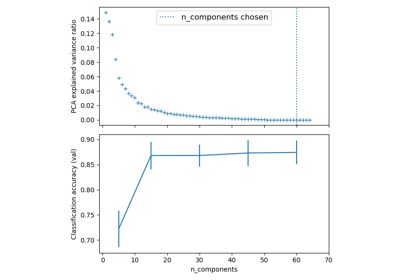
This figure motivates a stronger selection method than “keep 95% variance”:

1. Use explained variance to understand the geometry and form a reasonable range for $k$.
2. Evaluate several values of $k$ against the actual validation metric, latency, memory, and operational constraints.
3. Choose the smallest $k$ that meets the relevant quality requirement with acceptable uncertainty.

For a retrieval embedding pipeline, relevant downstream checks might include recall at $k$, latency, and index memory. For a perception classifier, they may include class-specific recall, calibration, and performance on rain, night, and occlusion slices. The right criterion follows the system objective, not PCA’s internal objective alone.

---

SVD: the practical route to PCA

The covariance approach is intuitive, but implementations commonly use singular value decomposition directly on the centered data matrix.

For a rank-$r$ centered matrix:

$$X_c=U\Sigma V^T$$

In the reduced or “thin” form, the shapes are:

$$U\in {\mathbb{R}}^{N\times r}$$ $$\Sigma \in {\mathbb{R}}^{r\times r}$$ $$V\in {\mathbb{R}}^{d\times r}$$

The diagonal entries of $\Sigma$, written ${\sigma }_1,\dots ,{\sigma }_r$, are singular values ordered from largest to smallest.

Substitute the SVD into the covariance definition:

$$C=\frac{1}{N-1}{X}_c^T{X}_c$$ $$C=\frac{1}{N-1}V{\Sigma }^T{U}^{T}U\Sigma V^T$$

Because the columns of $U$ are orthonormal, $U^{T}U=I$, so:

$$C=V\left(\frac{{\Sigma }^2}{N-1}\right)V^T$$

This identity is the bridge between SVD and PCA:

PCA quantity	SVD equivalent
Principal directions	Columns of $V$, the right singular vectors
PCA eigenvalues	${\lambda }_j=\frac{{\sigma }_j^2}{N-1}$
PCA scores	$Z=X_c{V}_k=U_k{\Sigma }_k$
Rank-$k$ reconstruction	${\hat{X}}_c=U_k{\Sigma }_k{V}_k^T$

The terminology is worth keeping precise. Singular values are not the covariance eigenvalues; their squares, adjusted by the covariance normalization constant, are the covariance eigenvalues.

Using the top $k$ SVD factors gives:

$$X_c\approx U_k{\Sigma }_k{V}_k^T$$

This is the best rank-$k$ approximation to $X_c$ under squared reconstruction error. In practice, direct SVD is numerically well-supported and avoids explicitly constructing $X_c^T{X}_c$, which can be undesirable for very high-dimensional features and worsens numerical conditioning.

One further implication follows from centering: the number of nonzero components cannot exceed:

$$\min (N-1,d)$$

If there are far more features than examples, PCA cannot produce more than $N-1$ nonzero variance directions after centering.

---

An interview-ready explanation

A concise answer can be structured around problem, geometry, computation, and caveat:

“PCA is a linear dimensionality-reduction method. After centering the data, I compute orthogonal directions that maximize projected variance, which is equivalent to minimizing squared reconstruction error for a chosen number of components. These directions are the eigenvectors of the covariance matrix, and their eigenvalues give the variance captured along each direction. In practice, I usually compute PCA with truncated SVD: the right singular vectors are the principal directions, and squared singular values are proportional to covariance eigenvalues. I select the number of components using explained variance as a diagnostic, then validate downstream task quality and resource trade-offs. PCA is unsupervised, so retaining variance does not guarantee retention of rare-class or label-relevant signal.”

Three mistakes to avoid in that explanation:

• “PCA selects the best original features.”
  No. PCA usually creates new features that are mixtures of the originals.

• “The first component is the most important feature.”
  It is the highest-variance direction, not automatically the most predictive or causally important direction.

• “A variance threshold proves the reduction is safe.”
  It only measures reconstruction of the input representation. Downstream and slice-level evaluation remain necessary.

---

Key takeaways

Eigenvectors are directions that a matrix scales without rotating away from their span; eigenvalues quantify the scaling. For PCA, the covariance matrix’s eigenvectors become orthogonal principal directions, and its eigenvalues equal the data variance along those directions.

With centered row-wise data:

$$X_c\in {\mathbb{R}}^{N\times d}$$

the top principal directions are stored in:

$$V_k\in {\mathbb{R}}^{d\times k}$$

and the reduced representation is:

$$Z=X_c{V}_k\in {\mathbb{R}}^{N\times k}$$

SVD provides the practical implementation:

$$X_c=U\Sigma V^T$$

The right singular vectors in $V$ are the PCA directions, while covariance eigenvalues are proportional to squared singular values. Finally, explained variance helps choose a candidate component count, but the correct final choice depends on downstream quality, safety slices, latency, and memory.

Next, you will move from the geometry of a model’s representation to its training mechanics: using the chain rule to compute gradients and explain gradient-based parameter updates.