Tight-Binding Model: 1D & 2D s-Orbitals

Hello! Welcome back to our course.

In our first lesson, we mapped out the geometric stage for electrons in a crystal by constructing Brillouin zones and identifying their high-symmetry points. We learned the where—the k-space coordinates that are important for describing electron states.

Today, we transition from this geometry to the physics that plays out on that stage. We will calculate the energy of electrons as a function of their wavevector, the famous band dispersion relation $E(\mathbf{k})$. To do this, we will develop one of the most powerful and intuitive pictures of electronic structure: the tight-binding model. This lesson will equip you to set up and solve the tight-binding Hamiltonian for simple lattices, which is a cornerstone for understanding the electronic properties of most materials.

Our goal is to derive the band dispersions for electrons hopping on 1D and 2D square lattices, assuming they occupy atomic s-orbitals.

1. The Tight-Binding Approximation: From Atoms to Crystals

The tight-binding model starts from the opposite philosophical standpoint to the nearly-free electron model. Instead of viewing electrons as plane waves slightly perturbed by the crystal potential, we imagine them as being tightly bound to their parent atoms. The crystal's electronic states then emerge from the interactions between these localized atomic orbitals. This is also known as the Linear Combination of Atomic Orbitals (LCAO) method.

Your familiarity with quantum mechanics, particularly with basis states and Hamiltonians, will be very useful here. The core idea is to build a Hamiltonian matrix using a basis of atomic orbitals and then find its eigenvalues.

Let's begin with a video that provides an excellent conceptual introduction to the model.

Constructing the Wavefunction and Hamiltonian

As the video introduced, we build our crystal wavefunctions from atomic orbitals. From your study of Bloch's theorem, you know that a wavefunction in a periodic potential must have the form ${\psi }_{\mathbf{k}}(\mathbf{r})=e^{i\mathbf{k}\cdot \mathbf{r}}{u}_{\mathbf{k}}(\mathbf{r})$, where $u_{\mathbf{k}}(\mathbf{r})$ has the periodicity of the lattice. A brilliant way to construct a function that automatically satisfies this theorem is to build a Bloch sum of atomic orbitals:

$${\psi }_{\mathbf{k}}(\mathbf{r})=\frac{1}{\sqrt{N}}\sum _{\mathbf{R}}{e}^{i\mathbf{k}\cdot \mathbf{R}}\varphi (\mathbf{r}-\mathbf{R})$$

Here, $N$ is the number of atoms, $\mathbf{R}$ are the lattice vectors, and $\varphi (\mathbf{r}-\mathbf{R})$ is the atomic orbital (e.g., an s-orbital) centered at site $\mathbf{R}$. Our goal is to find the energy of this state, $E(\mathbf{k})$, by solving the Schrödinger equation $H{\psi }_{\mathbf{k}}=E(\mathbf{k}){\psi }_{\mathbf{k}}$. The most direct way is to calculate the expectation value of the Hamiltonian:

$$E(\mathbf{k})=⟨{\psi }_{\mathbf{k}}|H|{\psi }_{\mathbf{k}}⟩$$

To make this calculation tractable, we make two critical simplifying assumptions:

1. Orthogonal Orbitals: We assume the atomic orbitals on different sites are orthogonal: $\int {\varphi }^{\ast }(\mathbf{r}-\mathbf{R})\varphi (\mathbf{r}-{\mathbf{R}}^{\prime })d^{3}r={\delta }_{\mathbf{R},{\mathbf{R}}^{\prime }}$. This is a strong approximation, as orbitals do overlap, but it simplifies the math considerably without losing the essential physics.
2. Hamiltonian Matrix Elements: We don't calculate the matrix elements from first principles. Instead, we parameterize them:
   • On-site energy ($ϵ$): The energy to have an electron at site $\mathbf{R}$ is $⟨\mathbf{R}|H|\mathbf{R}⟩=ϵ$. This is essentially the atomic energy level, shifted by the potential of the surrounding crystal. For a lattice of identical atoms, this is constant.
   • Hopping integral ($-t$): The energy associated with an electron "hopping" between nearest-neighbor sites $\mathbf{R}$ and ${\mathbf{R}}^{\prime }$ is $⟨{\mathbf{R}}^{\prime }|H|\mathbf{R}⟩=-t$. The parameter $t$ is positive, and the negative sign is a convention indicating that hopping lowers the system's energy.
   • All other matrix elements (for non-nearest neighbors) are set to zero.

The following video segment walks through this setup in detail. It uses the notation ${ϵ}_0$ for on-site energy and $J$ for the hopping parameter, which corresponds to our $t$.

2. Deriving the Band Dispersion

With the Hamiltonian and the Bloch-sum wavefunction defined, we can now derive the dispersion relation. A very elegant way to arrive at the general result is presented in the following document.

The key result from this reading is the general dispersion relation for a single s-band:

$$E(\mathbf{k})=ϵ+\sum _{\mathbf{\tau }}{e}^{i\mathbf{k}\cdot \mathbf{\tau }}\gamma (|\mathbf{\tau }|)$$

Here, the sum is over the nearest-neighbor vectors $\mathbf{\tau }$, and $\gamma (|\mathbf{\tau }|)$ is the overlap integral, which we will set to $-t$. For an isotropic system where all nearest-neighbor distances are the same, this simplifies to:

$$E(\mathbf{k})=ϵ-t\sum _{\mathbf{\tau }}{e}^{i\mathbf{k}\cdot \mathbf{\tau }}$$

Let's now apply this powerful formula to our specific cases.

2.1 The 1D Chain

For a 1D chain with lattice constant $a$, an atom at position $x=na$ has two nearest neighbors, at $(n-1)a$ and $(n+1)a$. The nearest-neighbor vectors are therefore $\mathbf{\tau }=a$ and $\mathbf{\tau }=-a$.

Plugging this into our general formula (and using a scalar $k$):

$$E(k)=ϵ-t\left(e^{ika}+e^{-ika}\right)$$

Using Euler's formula, $e^{ix}+e^{-ix}=2\cos (x)$, we arrive at the dispersion for the 1D tight-binding chain:

$$E(k)=ϵ-2t\cos (ka)$$

The video below confirms this result using a slightly different but equivalent method.

Let's visualize this result.

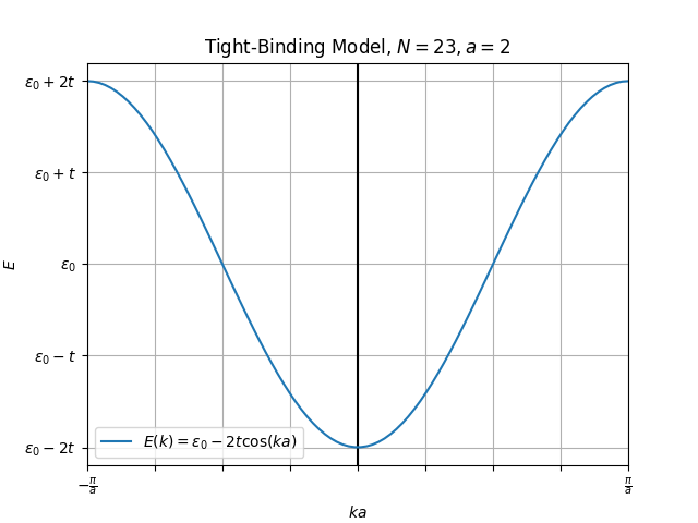
From the plot, we can see that the electron energies are confined to a continuous band of width $4t$. The minimum energy is $ϵ-2t$ at $k=0$ (the $\Gamma$ point), and the maximum is $ϵ+2t$ at $k=\pm \pi /a$ (the Brillouin zone edge). The hopping parameter $t$, which reflects the strength of the orbital overlap, directly controls the bandwidth.

Test your understanding!

Consider two 1D materials, A and B, made of the same atoms but with different lattice constants, $a_A<a_B$. How would you expect the hopping parameter $t$ and the bandwidth to compare between the two materials?

Show answer

Since the atoms in material A are closer together, their atomic orbitals will have a greater overlap. This corresponds to a larger hopping parameter, $t_A>t_B$. Consequently, the bandwidth, which is $4t$, will be wider for material A. This is a general principle: stronger interaction between orbitals leads to wider energy bands.

2.2 The 2D Square Lattice

Now we extend this to a 2D square lattice with lattice constant $a$. An atom at position $\mathbf{R}=(n_{x}a,n_{y}a)$ has four nearest neighbors. The nearest-neighbor vectors $\mathbf{\tau }$ are:

• $(a,0)$
• $(-a,0)$
• $(0,a)$
• $(0,-a)$

The wavevector is now a 2D vector $\mathbf{k}=(k_x,k_y)$. Applying our general formula:

$$E(k_x,k_y)=ϵ-t\left(e^{i{k}_{x}a}+e^{-i{k}_{x}a}+e^{i{k}_{y}a}+e^{-i{k}_{y}a}\right)$$

This simplifies beautifully to:

$$E(k_x,k_y)=ϵ-2t\left(\cos (k_{x}a)+\cos (k_{y}a)\right)$$

The following resource provides a very compact derivation of this result. Your background in QFT will make the notation immediately familiar, although the derivation itself doesn't require the full second quantization machinery.

Plotting the full $E(k_x,k_y)$ requires a 3D plot. More practically, we plot the dispersion along the high-symmetry paths we defined in the last lesson: $\Gamma \to X\to M\to \Gamma$.

• $\Gamma$ point: $\mathbf{k}=(0,0)$. $E(\Gamma )=ϵ-2t(\cos 0+\cos 0)=ϵ-4t$. (Band minimum)
• $X$ point: $\mathbf{k}=(\pi /a,0)$. $E(X)=ϵ-2t(\cos \pi +\cos 0)=ϵ-2t(-1+1)=ϵ$.
• $M$ point: $\mathbf{k}=(\pi /a,\pi /a)$. $E(M)=ϵ-2t(\cos \pi +\cos \pi )=ϵ-2t(-1-1)=ϵ+4t$. (Band maximum)

The total bandwidth in this case is $8t$.

Conclusion

In this lesson, we built our first model of electronic band structure. By starting with localized atomic orbitals and making a few key approximations, we derived the energy dispersion relation for electrons in a periodic potential.

Key Takeaways:

• The tight-binding model (or LCAO) describes electronic bands as arising from the hopping of electrons between localized atomic orbitals.
• The model is governed by two main parameters: the on-site energy $ϵ$ and the nearest-neighbor hopping integral $t$.
• The general dispersion is given by $E(\mathbf{k})=ϵ-t{\sum }_{\mathbf{\tau }}{e}^{i\mathbf{k}\cdot \mathbf{\tau }}$, where the sum is over nearest-neighbor vectors.
• For a 1D chain, this gives $E(k)=ϵ-2t\cos (ka)$ with a bandwidth of $4t$.
• For a 2D square lattice, this gives $E(k_x,k_y)=ϵ-2t(\cos (k_{x}a)+\cos (k_{y}a))$ with a bandwidth of $8t$.

You are now equipped with the fundamental tools to calculate band structures for simple Bravais lattices. This method is surprisingly powerful and forms the basis for understanding a vast range of materials.

Preview of the Next Lesson: We will apply the tight-binding formalism to a non-Bravais lattice: the 2D honeycomb lattice, the structure of graphene. This will require a slightly more sophisticated setup (a 2x2 Hamiltonian) and will lead us to one of the most exciting phenomena in modern condensed matter physics: the emergence of massless Dirac electrons.