Dirac Points in Graphene: A Tight-Binding Approach

Recommended resources

The freely available resources this lesson will direct you to.

Hello! Welcome back to our study of electronic band structures.

In the last lesson, we successfully applied the tight-binding model to simple Bravais lattices like the 1D chain and the 2D square lattice. We saw how the hopping of electrons between identical, localized orbitals on a periodic grid gives rise to energy bands with a characteristic cosine-like dispersion.

Today, we take a significant step forward by applying this model to a non-Bravais lattice: the 2D honeycomb lattice of graphene. This structure, composed of a triangular Bravais lattice with a two-atom basis, requires a slightly more sophisticated approach. Instead of a single scalar equation for the energy, we will need to construct and diagonalize a 2x2 Hamiltonian matrix. This richer mathematical structure leads to one of the most celebrated results in modern condensed matter physics: the emergence of linearly dispersing, "massless" electronic states called Dirac fermions.

Our goal is to derive this famous band structure and understand why these unique Dirac points appear at the Fermi level.

1. The Honeycomb Lattice: A Two-Atom Basis

Unlike the square lattice, the honeycomb lattice is not a Bravais lattice. You cannot get from one atom to all other atoms by translation with a single set of primitive vectors. The key is to recognize it as a triangular Bravais lattice with a two-atom basis.

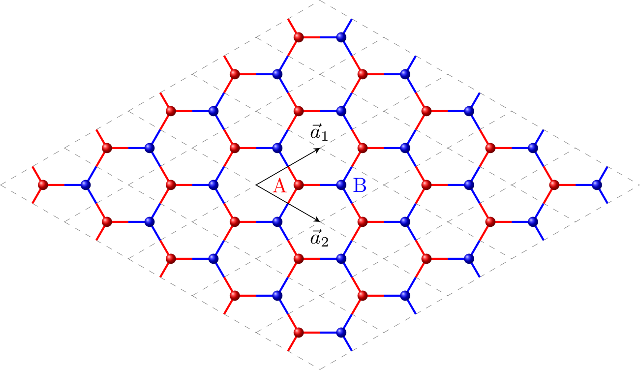
2D Honeycomb Lattice with Sublattices and Primitive Vectors — A 2D honeycomb lattice, showing the two inequivalent sublattices, A (red) and B (blue). The vectors $\mathbf{a}_1$ and $\mathbf{a}_2$ (not shown in this image, but defined in the text) are the primitive vectors of the underlying triangular Bravais lattice, while vectors like $\boldsymbol{\delta}_1, \boldsymbol{\delta}_2, \boldsymbol{\delta}_3$ connect an A-site to its nearest-neighbor B-sites.

This means every unit cell contains two carbon atoms, which we label A and B. As you can see in the image, any atom on the 'A' sublattice is surrounded by three 'B' atoms, and vice versa. This A-B distinction is the crucial new element compared to our previous lesson.

2. Justification: Why only $p_{z}$ Orbitals?

A carbon atom has four valence electrons in the $2 s$ and $2 p$ orbitals. A full tight-binding model would be complex. However, in graphene, three of these electrons ( $2 s, 2 p_{x}, 2 p_{y}$ ) hybridize to form strong, in-plane $σ$ -bonds (called $s p^{2}$ hybridization). These bonds are responsible for the rigid structure of graphene, and the corresponding electronic states lie at very high binding energies, far from the Fermi level.

This leaves one electron per atom in the out-of-plane $p_{z}$ orbital. These orbitals overlap to form weaker $π$ -bonds, and it is these $π$ -electrons that are responsible for the electronic conduction and the fascinating low-energy physics of graphene. Therefore, we can build an excellent effective model by considering only one $p_{z}$ orbital per carbon atom.

The following video explains this separation of energy scales beautifully.

Calculating the band structure of graphene

The video 'Calculating the band structure of graphene' by Professor Nano provides a detailed look at the orbital character of the bands.

Please watch from 15:47 to 18:24. Focus on how the plot shows that the bands crossing the Fermi level are composed almost exclusively of p_z orbital character, justifying our simplified model.

3. The 2x2 Tight-Binding Hamiltonian

Because we have two atoms (A and B) in our basis, our wavefunction in the unit cell must be a two-component "spinor", representing the amplitude of the electron on the A site and the B site.

Ψ_{k} = (c_{A} (k) c_{B} (k))

Consequently, the Bloch Hamiltonian $h (k)$ will be a 2x2 matrix. Its elements are determined by the on-site energies and the hopping between orbitals.

$h_{AA}$ and $h_{B B}$ : The on-site energies. Since both sites are carbon atoms, their energies are identical. We can set this energy to zero, as it only shifts the entire band structure up or down. So, $h_{AA} = h_{B B} = 0$ .
$h_{A B}$ and $h_{B A}$ : The hopping terms. We'll consider only nearest-neighbor hopping with strength $- t$ . An electron on a B-site can hop to three neighboring A-sites, and vice versa.

Your familiarity with second quantization from QFT will make the following derivation particularly transparent. The PDF below sets up the Hamiltonian in second quantization and transforms it to k-space to find the Bloch Hamiltonian.

Tutorial 1 - Graphene

The tutorial 'Tutorial 1 - Graphene' from the Weizmann Institute provides a concise and elegant derivation of the Bloch Hamiltonian for graphene.

Please read the section '2 Graphene' (pages 2-3), up to the definition of the Bloch Hamiltonian h. Pay close attention to how the two-component vector ψ(k) is defined and how the off-diagonal term f(k) arises from summing the phase factors for hopping to the three nearest neighbors.

From the reading, the Bloch Hamiltonian is:

h (k) = (0 f^{*} (k) f (k) 0) with f (k) = - t i = 1 \sum 3 e^{i k \cdot δ_{i}}

where $δ_{i}$ are the three vectors connecting an A-site to its nearest-neighbor B-sites.

The eigenvalues of this matrix are found easily:

det (h (k) - E \cdot I) = det (- E f^{*} (k) f (k) - E) = E^{2} - ∣ f (k) ∣^{2} = 0

This gives the energy dispersion relation for graphene's two bands:

E_{\pm} (k) = \pm ∣ f (k) ∣ = \pm t 3 + 2 cos (3 k_{y} a) + 4 cos (\frac{3}{2} k_{y} a) cos (\frac{3}{2} k_{x} a)

where $a$ is the C-C distance.

Graphene and Band Structure — The electronic band structure of graphene. On the left, the honeycomb atomic lattice. In the center, a sketch of the first Brillouin zone showing the high-symmetry points Γ, M, and the inequivalent corners K and K'. On the right, the 3D plot of the energy bands E(k), showing that the upper (conduction) and lower (valence) bands touch at the K and K' points, forming what are known as Dirac cones.

4. Emergence of Dirac Points

The most striking feature of this band structure is that the two bands touch at specific points. These are the points where the band gap closes, i.e., $E_{\pm} (k) = 0$ . This occurs when $f (k) = 0$ . Solving this condition reveals that the band-touching points are precisely the six corners of the hexagonal Brillouin zone. These six corners are not all independent; they form two inequivalent sets of three, labeled the K and K' points.

Near these special points, the physics becomes incredibly interesting. Let's analyze the dispersion in the vicinity of a K point by setting $k = K + q$ , where $q$ is a small momentum deviation. A Taylor expansion of $f (k)$ around $K$ shows that, to first order, $f (K + q)$ is linear in $q$ .

The following video provides a fantastic, comprehensive derivation of the band structure and a detailed analysis of the behavior near the K points.

GRAPHENE, DIRAC CONES, KLEIN TUNNELING

The video 'GRAPHENE, DIRAC CONES, KLEIN TUNNELING' from the 'Topological quantum matter' series clearly walks through the entire process, from setting up the Hamiltonian to analyzing the low-energy effective theory.

First, watch from 05:26 to 12:36. This section derives the 2x2 Bloch Hamiltonian and solves for the band structure, confirming the result we derived above. Then, watch from 15:24 to 19:32. This part is crucial: it shows the linearization of the Hamiltonian around the K and K' points, resulting in the famous Dirac Hamiltonian.

As the video explains, after linearization and a suitable rotation of coordinates, the effective Hamiltonian near the K point takes the form:

h (q) \approx ℏ v_{F} (q_{x} σ_{x} + q_{y} σ_{y}) = ℏ v_{F} q \cdot σ

Here, $v_{F} \approx 1 0^{6} m/s$ is the Fermi velocity, and $σ_{x}, σ_{y}$ are the Pauli matrices acting in the (A, B) sublattice space. This internal, two-level degree of freedom is called pseudospin.

This Hamiltonian is formally identical to the 2D Dirac equation for a massless relativistic particle, with the speed of light $c$ replaced by the Fermi velocity $v_{F}$ . This is a profound result: the collective behavior of non-relativistic electrons hopping on a honeycomb lattice gives rise to emergent quasiparticles that behave like massless Dirac fermions.

The energy spectrum for this Hamiltonian is:

E_{\pm} (q) \approx \pm ℏ v_{F} q_{x}^{2} + q_{y}^{2} = \pm ℏ v_{F} ∣ q ∣

This is a linear dispersion relation, forming the iconic 'Dirac cones' at the K and K' points.

Test your understanding!

Imagine we break the symmetry between the A and B sublattices, for example, by using a substrate that interacts differently with the two sites. This would give the A and B sites different on-site energies, say $+ Δ$ and $- Δ$ . How would this modify the 2x2 Bloch Hamiltonian, and what would the energy be exactly at the K point ( $q = 0$ )?

Show answer

The diagonal elements of the Hamiltonian would no longer be zero. The Hamiltonian would become:

h (k) = (Δ f^{*} (k) f (k) - Δ) = Δ σ_{z} + Re [f (k)] σ_{x} - Im [f (k)] σ_{y}

Exactly at the K point, $q = 0$ , so $f (K) = 0$ . The Hamiltonian simplifies to:

h (K) = (Δ 0 0 - Δ)

The energies are now $E = \pm Δ$ . The degeneracy is lifted, and a band gap of size $2Δ$ is opened at the Dirac point. The massless Dirac fermions have acquired a "mass".

This exact scenario of gap opening is not just a theoretical exercise; it's a real physical effect that is crucial for developing graphene-based electronics. The following video segments explain this and the underlying symmetry reasons for the stability of the Dirac points.

GRAPHENE, DIRAC CONES, KLEIN TUNNELING

Let's return to the 'Topological quantum matter' video to understand why the Dirac points are stable and how to break them.

Watch from 19:32 to 34:43. This advanced but important section explains that the Dirac points are protected by the combination of time-reversal and inversion (sublattice) symmetry. It then shows exactly the scenario from the exercise: breaking inversion symmetry (e.g., with an hBN substrate) opens a gap.

Conclusion

In this lesson, we tackled the electronic structure of graphene, a non-Bravais lattice. This required us to upgrade our tight-binding machinery from a scalar equation to a 2x2 matrix formalism.

Key Takeaways:

The honeycomb lattice is a triangular Bravais lattice with a two-atom (A and B) basis.
The low-energy electronic properties are dominated by the $p_{z}$ orbitals, allowing for a simplified single-orbital-per-atom model.
The two-atom basis leads to a 2x2 Bloch Hamiltonian, resulting in two energy bands.
These bands touch at the K and K' points of the Brillouin zone. Undoped graphene is a semimetal with a zero density of states at the Fermi energy.
Near the K and K' points, the energy dispersion is linear, $E \propto ∣ q ∣$ , forming Dirac cones.
The low-energy effective Hamiltonian is that of massless 2D Dirac fermions, where the A-B sublattice degree of freedom acts as a pseudospin.
The gapless Dirac points are protected by symmetry. Breaking the sublattice symmetry (e.g., with a substrate) opens a band gap and gives the fermions an effective mass.

You have now derived one of the cornerstone results of modern condensed matter physics from the ground up.

Preview of the Next Lesson: We will shift from analytical derivations to practical computation. You will learn how to implement a tight-binding Hamiltonian in Python and numerically diagonalize it to plot the band structure for any given lattice, including the graphene dispersion we derived today.