Deriving Logistic Regression

Recommended resources

The freely available resources this lesson will direct you to.

Welcome to the fifth lesson in our course. In our previous session, we completed a full derivation of the Ordinary Least Squares (OLS) solution for linear regression, culminating in a closed-form equation for the optimal model parameters. This was a crucial first step, demonstrating how a learning problem can be solved analytically through geometric and calculus-based reasoning.

Today, we shift our focus from regression to classification—from predicting continuous values to assigning discrete labels. Our goal is to derive logistic regression from the sigmoid function and the principle of maximum likelihood estimation. You will see how we adapt the linear model for a classification context and why this adaptation necessitates a different approach to finding the optimal parameters. This lesson will highlight a fundamental contrast with linear regression: the absence of a simple, closed-form solution, which introduces the need for the iterative optimization methods that dominate modern machine learning.

From Regression to Classification: A Motivating Problem

In the last lesson, our model $y^= w^{T} x$ could produce any real-valued number, which was appropriate for predicting quantities like housing prices. But what if we want to solve a binary classification problem, such as determining if a tumor is malignant (class 1) or benign (class 0)?

A naive approach might be to use linear regression and simply threshold the output: if $y^> 0.5$ , predict 1; otherwise, predict 0. However, this method has two significant theoretical flaws:

The model's output, $w^{T} x$ , is unbounded. It can be much greater than 1 or less than 0, which makes it difficult to interpret as a probability.
The model is highly sensitive to outliers. A single data point far from the decision boundary can drastically alter the regression line and lead to a poor classification boundary.

The following video lecture from Stanford's CS229 course offers an excellent visual demonstration of why linear regression is ill-suited for classification tasks.

Locally Weighted & Logistic Regression | Stanford CS229: Machine Learning - Lecture 3 (Autumn 2018)

This segment clearly explains the pitfalls of applying linear regression to a classification problem and introduces the need for a hypothesis that constrains its output to be between 0 and 1.

Please watch the section from the beginning of the classification discussion. Pay close attention to the example where adding a single, non-ambiguous data point changes the decision boundary for the worse. This motivates the introduction of the sigmoid function.

The Logistic Regression Hypothesis

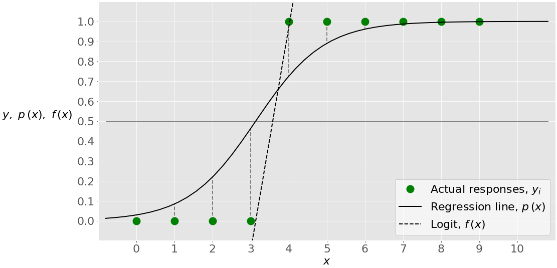
To address the shortcomings of a simple linear model, logistic regression introduces a non-linear transformation. We want to map the unbounded output of the linear part, $z = θ^{T} x$ , into a bounded interval of $(0, 1)$ so it can be interpreted as a probability. For this, we use the logistic function, also known as the sigmoid function:

g (z) = \frac{1}{1 + e ^{- z}}

This function has a characteristic "S" shape, asymptotically approaching 0 as $z \to - \infty$ and 1 as $z \to + \infty$ .

Our hypothesis for logistic regression, $h_{θ} (x)$ , is formed by applying the sigmoid function to a linear combination of the input features:

h_{θ} (x) = g (θ^{T} x) = \frac{1}{1 + e ^{- θ^{T} x}}

We interpret this output as the estimated probability that the label $y$ is 1, given the input $x$ and parameters $θ$ :

P (y = 1∣ x; θ) = h_{θ} (x)

The image below visualizes this relationship. The dashed line is the linear function $θ^{T} x$ (labeled Logit, f(x)), and the solid S-shaped curve is the resulting probability $h_{θ} (x)$ (labeled Regression line, p(x)), which is used to model the binary outcomes (the green dots y_i).

The logistic regression model. The linear function $\mathbf{\theta}^T\mathbf{x}$ is transformed by the sigmoid function to produce a probability between 0 and 1, which is then fitted to the binary target data.

Deriving the Model via Maximum Likelihood Estimation

In the previous lesson, we found the optimal parameters for linear regression by minimizing the sum of squared errors. Here, we will use a more general and powerful principle you were briefly introduced to: Maximum Likelihood Estimation (MLE). The core idea of MLE is to choose the parameters $θ$ that make our observed data most probable.

Let's build the derivation step-by-step.

1. The Probabilistic Model

Since our target variable $y$ can only be 0 or 1, we can model it as a Bernoulli random variable. The probability mass function (PMF) for a single observation $(y, x)$ can be written as:

If $y = 1$ : $P (y = 1∣ x; θ) = h_{θ} (x)$
If $y = 0$ : $P (y = 0∣ x; θ) = 1 - h_{θ} (x)$

A compact way to write this in a single equation is:

P (y ∣ x; θ) = (h_{θ} (x))^{y} (1 - h_{θ} (x))^{1 - y}

You can verify that this expression correctly gives $h_{θ} (x)$ when $y = 1$ and $1 - h_{θ} (x)$ when $y = 0$ . This clever formulation is central to the derivation.

The following segment of the Stanford lecture video provides a clear walkthrough of this probabilistic setup.

Locally Weighted & Logistic Regression | Stanford CS229: Machine Learning - Lecture 3 (Autumn 2018)

This part of the lecture carefully constructs the probabilistic assumption for logistic regression and derives the single, compact equation for the probability of an observation.

Watch from the start of the probabilistic assumption. Focus on how the two cases for y=1 and y=0 are combined into one expression using exponents.

2. The Likelihood and Log-Likelihood Functions

Assuming our $n$ training examples are independent and identically distributed (IID), the total likelihood of observing our entire dataset $(X, y)$ is the product of the individual probabilities:

L (θ) = P (y ∣ X; θ) = i = 1 \prod n P (y^{(i)} ∣ x^{(i)}; θ) = i = 1 \prod n (h_{θ} (x^{(i)}))^{y^{(i)}} (1 - h_{θ} (x^{(i)}))^{1 - y^{(i)}}

Our goal is to find the $θ$ that maximizes $L (θ)$ . As with linear regression's MLE justification, working with products is difficult. It is much easier to maximize the natural logarithm of the likelihood, the log-likelihood $ℓ (θ)$ , since the logarithm function is monotonic.

ℓ (θ) = lo g L (θ) = i = 1 \sum n lo g [(h_{θ} (x^{(i)}))^{y^{(i)}} (1 - h_{θ} (x^{(i)}))^{1 - y^{(i)}}]

Using the properties of logarithms ( $lo g (ab) = lo g a + lo g b$ and $lo g (a^{b}) = b lo g a$ ), we arrive at the log-likelihood function for logistic regression:

ℓ (θ) = i = 1 \sum n [y^{(i)} lo g h_{θ} (x^{(i)}) + (1 - y^{(i)}) lo g (1 - h_{θ} (x^{(i)}))]

This function is fundamental. In fact, its negative is the famous cross-entropy loss function, which we will explore in the next lesson.

For a rigorous, mathematical treatment of this derivation, please review the following resource.

Logistic regression - Maximum likelihood estimation

This article from StatLect provides a formal, step-by-step derivation of the logistic model's likelihood and log-likelihood functions.

Please read the first three sections: Model and notation The likelihood The log-likelihood

Finding the Optimal Parameters

Unlike linear regression, where setting the gradient of the loss to zero gave us the solvable Normal Equations, there is no closed-form solution for the $θ$ that maximizes $ℓ (θ)$ . The presence of the logarithm and sigmoid functions results in a system of transcendental equations that cannot be solved analytically.

Therefore, we must turn to iterative optimization algorithms, such as gradient ascent (or gradient descent on the negative log-likelihood). To use these methods, we need to compute the gradient of the log-likelihood function, $\nabla_{θ} ℓ (θ)$ .

The derivation involves applying the chain rule, making use of the convenient derivative of the sigmoid function: $g^{'} (z) = g (z) (1 - g (z))$ . Given your background in multivariable calculus, walking through this derivation is an excellent exercise.

The following notes provide a detailed, step-by-step derivation of the gradient.

Logistic Regression

These notes from a Stanford course meticulously derive the log-likelihood function and then compute its gradient with respect to the parameters.

Please read the following sections: Log Likelihood: Start at this section to see the log-likelihood construction again. Gradient of Log Likelihood: Read the introduction to this section, which presents the final gradient formula. Derivations: Carefully follow the detailed derivation using the chain rule. This is the mathematical core of today's lesson, breaking the complex derivative into manageable pieces.

After performing the derivation, we arrive at a beautifully simple expression for the partial derivative with respect to a single parameter $θ_{j}$ :

\frac{\partial}{\partial θ _{j}} ℓ (θ) = i = 1 \sum n (y^{(i)} - h_{θ} (x^{(i)})) x_{j}^{(i)}

This tells us how to update our parameters in a gradient ascent algorithm:

θ_{j} := θ_{j} + α i = 1 \sum n (y^{(i)} - h_{θ} (x^{(i)})) x_{j}^{(i)}

where $α$ is the learning rate.

Interestingly, this update rule looks identical to the one for linear regression! The crucial difference, of course, is the definition of the hypothesis $h_{θ} (x)$ . For linear regression, it was $θ^{T} x$ , while here it is $g (θ^{T} x)$ . This subtle but profound difference is what separates the two algorithms.

The final segment of the Stanford video discusses this optimization process and the fascinating similarity of the update rule.

Locally Weighted & Logistic Regression | Stanford CS229: Machine Learning - Lecture 3 (Autumn 2018)

This concluding segment brings everything together: formulating the log-likelihood, introducing gradient ascent for maximization, and discussing the final update rule.

Watch from the maximum likelihood section. Note the switch from minimization (gradient descent) to maximization (gradient ascent) and the lecturer's explanation of why the final update rule looks so familiar.

Conclusion

In this lesson, we have derived one of the most fundamental classification algorithms in machine learning from first principles. We bridged the gap between linear models and classification by introducing the sigmoid function and framed the learning problem within the powerful paradigm of Maximum Likelihood Estimation.

Here are the key takeaways:

Hypothesis: Logistic regression models the probability of a positive class using the sigmoid function applied to a linear input: $h_{θ} (x) = g (θ^{T} x)$ .
Probabilistic Foundation: The model is derived by assuming the binary outcome follows a Bernoulli distribution, and its parameters are found by maximizing the log-likelihood of the training data.
Log-Likelihood Function: The MLE principle naturally leads to the log-likelihood function $ℓ (θ) = \sum [y lo g h_{θ} (x) + (1 - y) lo g (1 - h_{θ} (x))]$ .
Gradient-Based Optimization: Unlike OLS linear regression, logistic regression has no closed-form solution. We must use iterative methods like gradient ascent, for which we derived the gradient of the log-likelihood function. The resulting update rule is $θ_{j} := θ_{j} + α \sum (y^{(i)} - h_{θ} (x^{(i)})) x_{j}^{(i)}$ .

You now understand not just what logistic regression is, but why it takes the form it does. In our next lesson, we will formally define the cross-entropy loss function—the negative of the log-likelihood you derived today—and explore its deep connection to information theory, providing another layer of theoretical justification for its use in classification.