Cross-Entropy Loss: Theory and Information-Theoretic Interpretation

Welcome to the final lesson of our module on the Core Concepts of Supervised Learning. In our last session, we conducted a thorough derivation of the logistic regression model, starting from the principle of Maximum Likelihood Estimation (MLE). This led us to the log-likelihood function, which we sought to maximize:

$$\ell (\theta )=\sum _{i=1}^n\left[y^{(i)}\log h_{\theta }({\mathbf{x}}^{(i)})+(1-y^{(i)})\log (1-h_{\theta }({\mathbf{x}}^{(i)}))\right]$$

We noted that maximizing this function is equivalent to minimizing its negative, a standard practice in optimization. Today, we will formally define this negative log-likelihood as the cross-entropy loss function. Our primary objective is to move beyond this purely optimization-based view and explain its deeper information-theoretic interpretation. This will provide a robust theoretical justification for why cross-entropy is the de facto standard loss function for classification tasks, connecting probability, optimization, and information theory.

From Log-Likelihood to Cross-Entropy Loss

In machine learning, the convention is to frame learning as a process of minimizing a loss or cost function. Therefore, instead of maximizing the log-likelihood, we minimize its negative. For a dataset of $n$ samples, the average negative log-likelihood gives us the binary cross-entropy loss function:

$$J(\theta )=-\frac{1}{n}\ell (\theta )=-\frac{1}{n}\sum _{i=1}^n\left[y^{(i)}\log (h_{\theta }({\mathbf{x}}^{(i)}))+(1-y^{(i)})\log (1-h_{\theta }({\mathbf{x}}^{(i)}))\right]$$

Let's analyze the contribution of a single data point to this loss. Let $\hat{y}=h_{\theta }(\mathbf{x})$ be the model's predicted probability for the positive class.

• If the true label is $y=1$, the loss is $-\log (\hat{y})$.
• If the true label is $y=0$, the loss is $-\log (1-\hat{y})$.

This behavior is visualized below.

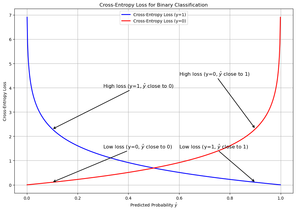
As the plot illustrates, the loss penalizes confident, incorrect predictions exponentially. If the true class is 1 ($y=1$) but the model predicts a probability close to 0 ($\hat{y}\to 0$), the loss $-\log (\hat{y})$ skyrockets. Conversely, a correct and confident prediction ($\hat{y}\to 1$) results in a loss close to zero. This intuitive behavior is desirable, but the true power and elegance of cross-entropy come from its roots in information theory.

An Information-Theoretic Perspective

To understand why this specific functional form is so fundamental, we need to take a detour into information theory, the mathematical study of the quantification, storage, and communication of information.

The following article from Eli Bendersky's website provides an excellent, bottom-up introduction to the key concepts we need. We will work through it step by step.

Let's summarize the key ideas you've just read about:

1. Information Content (Surprise): The information gained from observing an event with probability $p$ is $-{\log }_2(p)$. Unlikely events ($p\to 0$) are highly surprising and carry more information.

2. Entropy: The entropy of a probability distribution $P$, denoted $H(P)$, is the expected surprise. It's the average amount of information we get from one sample of the distribution. For a discrete distribution, it's calculated as:
   $H(P)=-{\sum }_i{p}_i{\log }_2(p_i)$
   Entropy can be interpreted as the minimum average number of bits required to encode a message drawn from distribution $P$.

3. Cross-Entropy: This is the crucial concept. Suppose the true data distribution is $P$, but we devise an encoding scheme based on an incorrect, estimated distribution $Q$. The average number of bits we will need to encode messages from $P$ using the code for $Q$ is the cross-entropy, $H(P,Q)$:
   $H(P,Q)=-{\sum }_i{p}_i{\log }_2(q_i)$
   It is the expected surprise when events are drawn from $P$, but we evaluate their surprise using the probabilities from $Q$.

The following short video from Aurélien Géron provides a brilliant analogy for these concepts using weather forecasts, which can help solidify your intuition.

The Connection to Machine Learning and KL Divergence

Now, let's tie this back to our classification problem.

• The true distribution $P$ is represented by the ground-truth labels. For a multi-class problem, a specific data point's true label is a one-hot vector, like [0, 1, 0, 0]. This is a distribution with no uncertainty—its entropy is zero.
• The predicted distribution $Q$ is the output of our model, typically from a softmax layer, like [0.1, 0.7, 0.15, 0.05].

The cross-entropy loss function is precisely $H(P,Q)$! It measures the average number of bits needed to encode the true labels when we use our model's predictions as our encoding scheme. We want to adjust our model parameters $\theta$ to make $Q$ as close to $P$ as possible, thereby minimizing this "average message length."

This brings us to a related concept: Kullback-Leibler (KL) Divergence. The cross-entropy $H(P,Q)$ is the cost of using code $Q$, while the entropy $H(P)$ is the cost of the optimal code. The difference between them is the "extra" cost, or wasted bits, due to using the suboptimal code $Q$. This extra cost is the KL Divergence.

$$D_{KL}(P||Q)=H(P,Q)-H(P)$$

Since $D_{KL}(P||Q)\ge 0$, this gives us the important inequality: $H(P,Q)\ge H(P)$. The cross-entropy is always greater than or equal to the true entropy, with equality holding if and only if $P=Q$.

Let's continue with the resources to formalize this.

The key insight for machine learning is that during training, the true data distribution $P$ is fixed. Therefore, its entropy $H(P)$ is a constant. As a result:

Minimizing $H(P,Q)$ with respect to model parameters is equivalent to minimizing $D_{KL}(P||Q)$.

This provides a powerful justification: training a classifier with cross-entropy loss is equivalent to minimizing the "distance" (in an information-theoretic sense, as KL-divergence is not a true metric) between the predicted probability distribution and the true one.

The following video provides another excellent summary of these relationships.

Binary vs. Categorical Cross-Entropy

Let's explicitly write out the cross-entropy for the two main types of classification.

1. Binary Cross-Entropy:
As we saw, for a single data point, the true distribution is $P=(y,1-y)$ and the predicted distribution is $Q=(\hat{y},1-\hat{y})$. The cross-entropy is:
$H(P,Q)=-[y\log (\hat{y})+(1-y)\log (1-\hat{y})]$
This is exactly one term in the loss function for logistic regression.

2. Categorical Cross-Entropy:
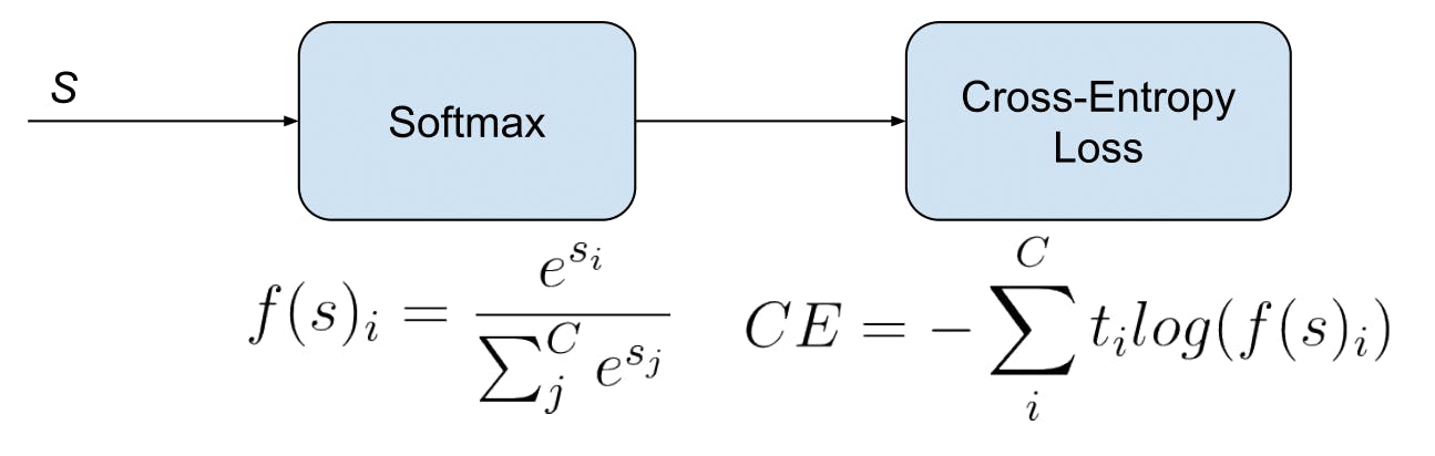
For multi-class classification with $C$ classes, the output of the model is typically a vector of probabilities from a Softmax function. The true label is a one-hot vector $\mathbf{y}$. The loss for a single sample is:
$H(\mathbf{y},\hat{\mathbf{y}})=-{\sum }_{i=1}^C{y}_i\log ({\hat{y}}_i)$
Since $\mathbf{y}$ is one-hot, only the term corresponding to the true class is non-zero. For example, if the true class is $k$, then $y_k=1$ and all other $y_i=0$, so the loss simplifies to $-\log ({\hat{y}}_k)$.

This entire process for multi-class classification is depicted below.

For a rigorous walkthrough of the generalization from binary to multi-class cross-entropy and its equivalence to maximizing the multinoulli log-likelihood, the following resource is invaluable.

Conclusion

In this lesson, we established a deep, multi-faceted understanding of the cross-entropy loss function. It is not merely an arbitrary choice that happens to work well; it is a principled objective derived from both probability theory and information theory.

Here are the key takeaways:

• Probabilistic View: Minimizing the cross-entropy loss is equivalent to Maximum Likelihood Estimation, i.e., finding the model parameters that make the observed data most probable.
• Information-Theoretic View: Cross-entropy measures the average number of bits required to encode the true data distribution using the model's predicted distribution. Minimizing it means making our model's predictions a more efficient code for the reality.
• Equivalence to KL Divergence: Since the entropy of the true data is constant, minimizing cross-entropy is equivalent to minimizing the KL divergence between the predicted and true probability distributions.
• Binary vs. Categorical: The familiar loss function from logistic regression is binary cross-entropy. For multi-class problems, we use categorical cross-entropy, which compares the model's softmax output to the one-hot encoded true label.

You have now completed the core theoretical foundations of supervised learning, from linear and logistic regression models to the loss functions that guide their training. In the next module, Optimization and Model Fitting, we will begin by formally comparing the loss functions we've seen (Mean Squared Error and Cross-Entropy). We will then dive deep into the primary algorithm used to minimize them: gradient descent.