Deriving OLS from Normal Equations

Welcome to our fourth lesson. In the previous session, we established the essential vocabulary of supervised learning: hypothesis spaces, parameters, and hyperparameters. We are now equipped to transition from abstract definitions to concrete application. This lesson marks our first deep dive into a specific learning algorithm, where we will derive the optimal parameters for a model from first principles.

Our focus will be on linear regression, a cornerstone of machine learning. The learning outcome for this lesson is to derive the ordinary least squares solution for linear regression from the normal equations. We will define a linear model, formulate an objective function based on minimizing squared error, and then use two powerful perspectives—one geometric and one based on calculus—to arrive at a closed-form solution for the model's parameters. This process will transform the abstract idea of a learning algorithm "searching" a hypothesis space into a precise, mathematical procedure.

The Linear Regression Model

Let's begin by formally defining our model. In linear regression, we assume the relationship between a set of input features and an output target is linear. For a single data example with $d$ features, $\mathbf{x}=[x_1,x_2,...,x_d{]}^T$, we predict the target value $\hat{y}$ using a linear combination of these features:

$$\hat{y}=w_0+w_1{x}_1+w_2{x}_2+\cdots +w_d{x}_d$$

Here, $w_1,...,w_d$ are the model parameters (weights) corresponding to each feature, and $w_0$ is the bias or intercept term.

To make the derivation cleaner, we can absorb the bias term $w_0$ into the weight vector. We do this by introducing an extra feature, $x_0$, that is always equal to 1 for every data point. Our feature vector becomes $\mathbf{x}=[x_0,x_1,...,x_d{]}^T=[1,x_1,...,x_d{]}^T$, and our parameter vector becomes $\mathbf{w}=[w_0,w_1,...,w_d{]}^T$. With this trick, the hypothesis is now a simple dot product:

$$\hat{y}={\mathbf{w}}^T\mathbf{x}$$

Now, let's extend this to our entire dataset. Suppose we have $n$ training examples. We can stack our feature vectors into a design matrix $\mathbf{X}$ of size $n\times (d+1)$, where each row corresponds to one training example. We can also stack our true target values into a vector $\mathbf{y}$ of size $n\times 1$.

$$\mathbf{X}=\left(\begin{array}{c}({\mathbf{x}}^{(1)}{)}^T\\ ({\mathbf{x}}^{(2)}{)}^T\\ ⋮\\ ({\mathbf{x}}^{(n)}{)}^T\end{array}\right)=\left(\begin{array}{cccc}1& x_1^{(1)}& \cdots & x_d^{(1)}\\ 1& x_1^{(2)}& \cdots & x_d^{(2)}\\ ⋮& ⋮& \ddots & ⋮\\ 1& x_1^{(n)}& \cdots & x_d^{(n)}\end{array}\right),\mathbf{y}=\left(\begin{array}{c}{y}^{(1)}\\ y^{(2)}\\ ⋮\\ y^{(n)}\end{array}\right)$$

Using this matrix notation, we can compute all $n$ predictions at once with a single matrix-vector multiplication:

$$\hat{\mathbf{y}}=\mathbf{Xw}$$

The following video lecture from Stanford's CS229 course provides an excellent overview of this notational setup, which is standard across machine learning.

The Cost Function: Ordinary Least Squares (OLS)

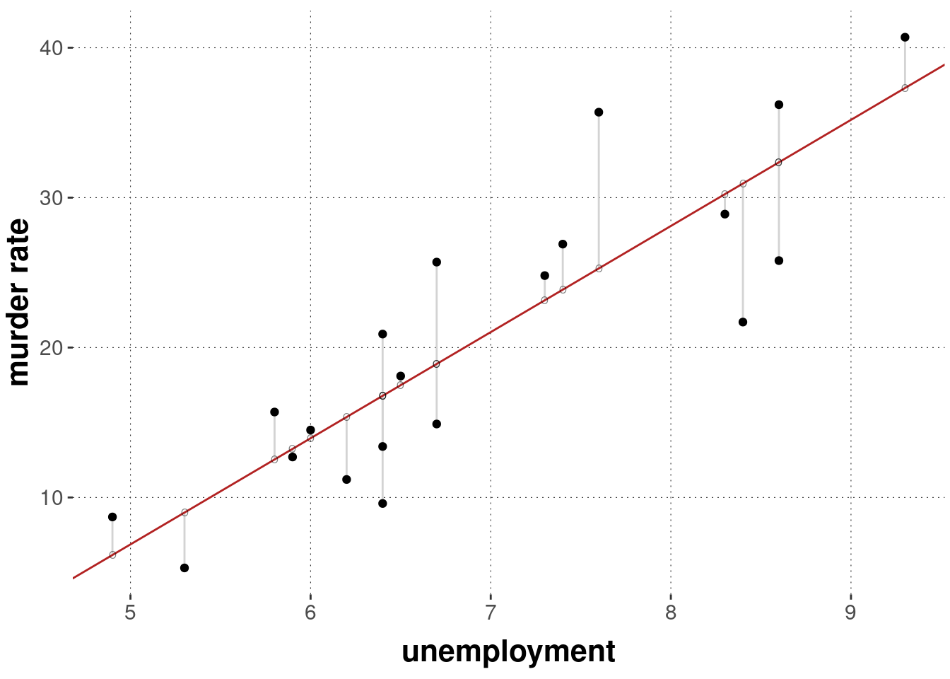
Our goal is to find the parameter vector $\mathbf{w}$ that makes our predictions $\hat{\mathbf{y}}$ as close as possible to the true values $\mathbf{y}$. We need a way to quantify the total error. In Ordinary Least Squares (OLS), we use the Sum of Squared Errors (SSE), also known as the Residual Sum of Squares (RSS).

The vector of errors, or residuals, is $\mathbf{e}=\mathbf{y}-\hat{\mathbf{y}}=\mathbf{y}-\mathbf{Xw}$. The SSE is the sum of the squares of these individual errors. In vector terms, this is the squared Euclidean norm (or L2 norm) of the residual vector:

$$L(\mathbf{w})=\sum _{i=1}^n(y^{(i)}-{\hat{y}}^{(i)}{)}^2=||\mathbf{y}-\hat{\mathbf{y}}|{|}^2=||\mathbf{y}-\mathbf{Xw}|{|}^2$$

Our optimization problem is therefore to find the $\mathbf{w}$ that minimizes this cost function:

$$\hat{\mathbf{w}}=\underset{\mathbf{w}}{\mathrm{argmin}}||\mathbf{y}-\mathbf{Xw}|{|}^2$$

This formulation is the heart of OLS. We are looking for the linear model that minimizes the squared vertical distances between the observed data points and the regression line, as illustrated below.

The Geometric Derivation of the Normal Equations

One of the most elegant ways to derive the solution is through geometric intuition. Your background in linear algebra will be particularly useful here.

The vector of predictions, $\hat{\mathbf{y}}=\mathbf{Xw}$, is a linear combination of the columns of the design matrix $\mathbf{X}$. This means that $\hat{\mathbf{y}}$ must lie within the column space of $\mathbf{X}$, denoted $\text{col}(\mathbf{X})$.

Our problem is to find a vector $\hat{\mathbf{y}}$ in $\text{col}(\mathbf{X})$ that is closest to our observed data vector $\mathbf{y}$. Geometrically, the vector in a subspace that is closest to an external point is the orthogonal projection of that point onto the subspace.

This means the residual vector, $\mathbf{e}=\mathbf{y}-\hat{\mathbf{y}}$, must be orthogonal to the entire column space of $\mathbf{X}$. For $\mathbf{e}$ to be orthogonal to $\text{col}(\mathbf{X})$, it must be orthogonal to every column in $\mathbf{X}$. This condition can be stated compactly using the transpose of $\mathbf{X}$:

$${\mathbf{X}}^T\mathbf{e}=0$$

Substituting $\mathbf{e}=\mathbf{y}-\mathbf{Xw}$, we get:

$${\mathbf{X}}^T(\mathbf{y}-\mathbf{X}\hat{\mathbf{w}})=0$$

Rearranging this gives us the Normal Equations:

$${\mathbf{X}}^T\mathbf{X}\hat{\mathbf{w}}={\mathbf{X}}^T\mathbf{y}$$

This is a remarkable result. We have transformed a complex minimization problem into a straightforward system of linear equations. The following video provides a concise walkthrough of this geometric derivation.

The Calculus Derivation of the Normal Equations

An alternative path to the same result is through multivariable calculus. Since you have a strong mathematical background, seeing the problem from this angle will reinforce the solution's validity. We start again with the cost function and find the point where its gradient is zero.

The cost function is $L(\mathbf{w})=||\mathbf{y}-\mathbf{Xw}|{|}^2$. Let's write this using the dot product definition of the squared norm, $||\mathbf{v}|{|}^2={\mathbf{v}}^T\mathbf{v}$.

$$L(\mathbf{w})=(\mathbf{y}-\mathbf{Xw}{)}^T(\mathbf{y}-\mathbf{Xw})$$

Expanding this expression:

$$L(\mathbf{w})=({\mathbf{y}}^T-(\mathbf{Xw}{)}^T)(\mathbf{y}-\mathbf{Xw})=({\mathbf{y}}^T-{\mathbf{w}}^T{\mathbf{X}}^T)(\mathbf{y}-\mathbf{Xw})$$ $$L(\mathbf{w})={\mathbf{y}}^T\mathbf{y}-{\mathbf{y}}^T\mathbf{Xw}-{\mathbf{w}}^T{\mathbf{X}}^T\mathbf{y}+{\mathbf{w}}^T{\mathbf{X}}^T\mathbf{Xw}$$

Note that ${\mathbf{w}}^T{\mathbf{X}}^T\mathbf{y}$ is a scalar, so it's equal to its own transpose: $({\mathbf{w}}^T{\mathbf{X}}^T\mathbf{y}{)}^T={\mathbf{y}}^T\mathbf{Xw}$. Thus, we can combine the two middle terms:

$$L(\mathbf{w})={\mathbf{y}}^T\mathbf{y}-2{\mathbf{w}}^T{\mathbf{X}}^T\mathbf{y}+{\mathbf{w}}^T{\mathbf{X}}^T\mathbf{Xw}$$

To find the minimum, we take the gradient of $L(\mathbf{w})$ with respect to $\mathbf{w}$ and set it to the zero vector. Using the following standard matrix calculus identities:

• ${\nabla }_{\mathbf{w}}({\mathbf{w}}^T\mathbf{a})=\mathbf{a}$
• ${\nabla }_{\mathbf{w}}({\mathbf{w}}^T\mathbf{Aw})=2\mathbf{Aw}$ (for symmetric $\mathbf{A}$; note ${\mathbf{X}}^T\mathbf{X}$ is symmetric)

We get:

$${\nabla }_{\mathbf{w}}L(\mathbf{w})=-2{\mathbf{X}}^T\mathbf{y}+2{\mathbf{X}}^T\mathbf{Xw}$$

Setting the gradient to zero:

$$-2{\mathbf{X}}^T\mathbf{y}+2{\mathbf{X}}^T\mathbf{X}\hat{\mathbf{w}}=0$$ $${\mathbf{X}}^T\mathbf{X}\hat{\mathbf{w}}={\mathbf{X}}^T\mathbf{y}$$

Once again, we arrive at the Normal Equations. The following lecture notes provide a rigorous, step-by-step walkthrough of both the geometric and calculus-based derivations.

The Closed-Form Solution

The Normal Equations give us a system of $d+1$ linear equations with $d+1$ unknowns (the elements of $\hat{\mathbf{w}}$). We can solve for $\hat{\mathbf{w}}$ directly.

If the matrix ${\mathbf{X}}^T\mathbf{X}$ is invertible, we can pre-multiply both sides by its inverse to isolate $\hat{\mathbf{w}}$:

$$({\mathbf{X}}^T\mathbf{X}{)}^{-1}({\mathbf{X}}^T\mathbf{X})\hat{\mathbf{w}}=({\mathbf{X}}^T\mathbf{X}{)}^{-1}{\mathbf{X}}^T\mathbf{y}$$ $$\mathbf{I}\hat{\mathbf{w}}=({\mathbf{X}}^T\mathbf{X}{)}^{-1}{\mathbf{X}}^T\mathbf{y}$$

This gives us the celebrated closed-form solution for Ordinary Least Squares:

$$\hat{\mathbf{w}}=({\mathbf{X}}^T\mathbf{X}{)}^{-1}{\mathbf{X}}^T\mathbf{y}$$

This equation is a significant result. It tells us that, unlike many other machine learning algorithms that require iterative optimization, we can calculate the optimal parameters for linear regression directly through a sequence of matrix operations.

The condition for this to work is that ${\mathbf{X}}^T\mathbf{X}$ must be invertible. This is true if and only if the columns of the design matrix $\mathbf{X}$ are linearly independent. In a machine learning context, this means you don't have redundant features (e.g., including a feature for temperature in Celsius and another for temperature in Fahrenheit) or more features than data points.

The text from Dive into Deep Learning provides a succinct summary of this final step.

Connection to Maximum Likelihood Estimation

Why the squared error? While it's computationally convenient, there's a deeper probabilistic justification. If we assume that the target variable $y$ is generated from a linear function of $\mathbf{x}$ plus some Gaussian (normal) noise, $y={\mathbf{w}}^T\mathbf{x}+ϵ$, where $ϵ\sim \mathcal{N}(0,{\sigma }^2)$, then the OLS solution is also the Maximum Likelihood Estimate (MLE) for $\mathbf{w}$.

In essence, under the assumption of Gaussian noise, the parameters $\mathbf{w}$ that are most likely to have generated our observed data $\mathbf{y}$ are exactly the same parameters that minimize the sum of squared errors. This provides a powerful theoretical justification for the OLS cost function.

You will explore MLE in more detail in a future lesson, but it is a key principle that connects probabilistic modeling and optimization in machine learning. The section on "The Normal Distribution and Squared Loss" in the Dive into Deep Learning resource (ID LINK) explains this connection well if you wish to read ahead.

Conclusion

In this lesson, we have performed our first end-to-end derivation of a machine learning model's training process. We moved from the abstract concept of finding the "best" parameters to a concrete, analytical solution.

Key takeaways from this lesson include:

• Model Formulation: Linear regression can be expressed compactly using matrix notation as $\hat{\mathbf{y}}=\mathbf{Xw}$.
• Cost Function: The OLS objective is to minimize the Sum of Squared Errors (SSE), which is equivalent to minimizing the squared L2 norm of the residual vector, $||\mathbf{y}-\mathbf{Xw}|{|}^2$.
• The Normal Equations: By using either geometric arguments (orthogonality of residuals) or calculus (setting the gradient to zero), we can transform the minimization problem into a system of linear equations: ${\mathbf{X}}^T\mathbf{X}\hat{\mathbf{w}}={\mathbf{X}}^T\mathbf{y}$.
• The Closed-Form Solution: When the features are linearly independent, the normal equations can be solved directly, yielding the unique OLS solution: $\hat{\mathbf{w}}=({\mathbf{X}}^T\mathbf{X}{)}^{-1}{\mathbf{X}}^T\mathbf{y}$.

You now have a complete theoretical understanding of how to find the optimal parameters for a linear regression model. In our next lesson, we will move to classification problems and derive the logistic regression model. This will provide a crucial contrast, as we will see that logistic regression does not have a closed-form solution, forcing us to explore the iterative optimization methods that are far more common in modern machine learning.