Understanding Model Components: Hypotheses, Parameters, and Hyperparameters

Welcome to our third lesson. In our previous discussion, we created a high-level map of the machine learning landscape, distinguishing between the supervised, unsupervised, and reinforcement learning paradigms. We are now prepared to zoom into the most common of these—supervised learning—and dissect its fundamental components.

The goal of this lesson is to define three essential concepts that form the theoretical bedrock of model building: hypothesis spaces, model parameters, and hyperparameters. Understanding the precise roles of and distinctions between these terms is critical for the overarching process of model selection—the methodical procedure of choosing a function that not only fits your data but also generalizes well to new, unseen examples.

The Anatomy of a Learning Problem

At its core, supervised learning is a problem of function approximation. We assume there is some true, unknown target function, $f:X\to Y$, that perfectly maps inputs to outputs. We don't have access to this function directly. Instead, we have a set of training examples, $(x^{(1)},y^{(1)}),...,(x^{(n)},y^{(n)})$, which are noisy samples from this true function.

The task of a learning algorithm is to use these training examples to produce a final hypothesis, $h$, which is our best guess at the true target function $f$. The algorithm selects this hypothesis from a predefined set of possibilities. This entire process is visualized in the following flowchart.

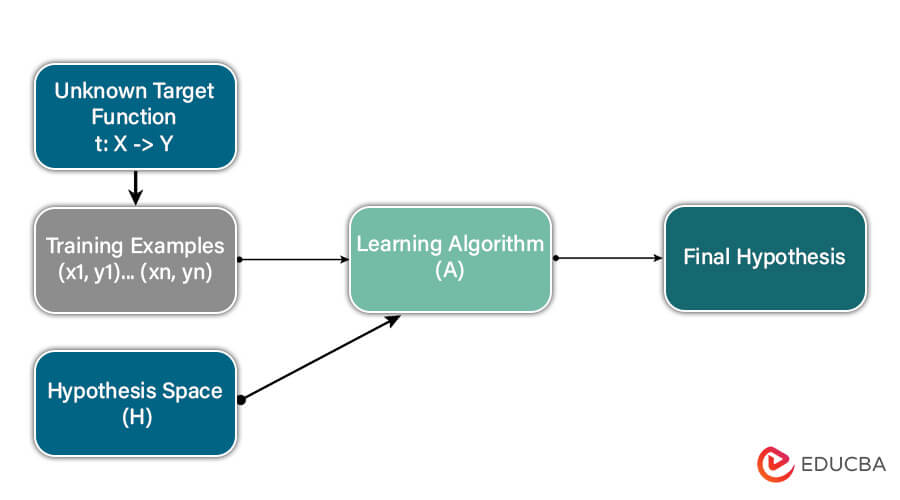
Let's now formally define the key components of this process.

Hypothesis Space: The Universe of Possibilities

Before any learning can occur, we must first decide on the class of functions our algorithm is allowed to consider. This pre-defined "universe" of all candidate functions is called the hypothesis space, denoted by $H$.

A hypothesis ($h\in H$) is simply one specific function from this space. For example, if we are predicting house prices from their size, one hypothesis might be $price=100\times size+50000$, while another might be $price=150\times size+10000$.

The choice of learning algorithm implicitly defines the hypothesis space.

• If you choose to use linear regression, your hypothesis space $H$ is the set of all linear functions of the input features.
• If you choose to use decision trees, your hypothesis space $H$ is the set of all possible trees you can form using your features.

The following video provides an excellent formal introduction to the concept of a hypothesis space. It explains how the choice of features and the "language" (the class of functions) together define the space from which a learning algorithm must select its final model.

As the video illustrates, the hypothesis space can be astronomically large. Given your background in computer science, you can think of the hypothesis space as being analogous to the set of all valid programs that can be expressed in a given programming language. A learning algorithm's job is to search this vast space for a single "program" (the final hypothesis) that best fits the training data according to some objective.

Model Parameters vs. Hyperparameters

Now that we have defined the space of possible models, we need to distinguish between the two types of "knobs" we can turn: those the algorithm adjusts automatically and those we must set manually.

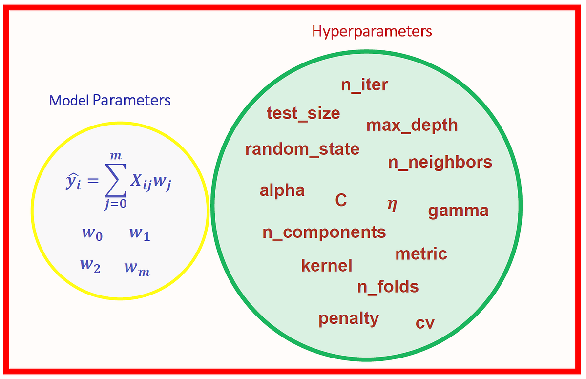
Model Parameters (e.g., $\theta$)

Model parameters are the variables that the learning algorithm learns from the training data. They are internal to the model and are the direct output of the training process. Once these parameters are learned, they define a specific hypothesis $h$ from the hypothesis space $H$.

Consider a simple linear regression model: $h_{\theta }(x)={\theta }_0+{\theta }_{1}x$.

• The hypothesis space is the set of all straight lines.
• The model parameters are the coefficients ${\theta }_0$ (the intercept) and ${\theta }_1$ (the slope).
• The learning algorithm's task is to find the specific values of ${\theta }_0$ and ${\theta }_1$ that make the line best fit the training data.

Hyperparameters (e.g., $\lambda$)

Hyperparameters, in contrast, are configuration settings that are set by you before the learning process begins. They are external to the model and are not learned from the data. Instead, they control how the learning algorithm finds the optimal model parameters.

Consider a regularized linear regression model (which we'll study in detail later). The objective is to find parameters $\theta$ that not only fit the data but also have small values to prevent overfitting.

• The model parameters are still the coefficients ${\theta }_j$.
• A crucial hyperparameter is the regularization strength, $\lambda$. This value controls the penalty for large parameter values. You must choose a value for $\lambda$ before you start training. Different values of $\lambda$ will cause the algorithm to learn different model parameters $\theta$.

The following resources provide formal, academic definitions that clearly delineate these concepts.

For a more formal and in-depth treatment, the following paper on hyperparameter optimization (HPO) defines these terms from first principles.

The Interplay: Model Selection

The ultimate goal is not just to find any model, but to find the best one. This process, called model selection, involves making choices at all three levels we've discussed:

1. Choosing the Hypothesis Space: Do we use a linear model, a polynomial model, a decision tree?
2. Tuning the Hyperparameters: If we choose a polynomial model, what should its degree be? If we use regularization, what should $\lambda$ be?
3. Learning the Model Parameters: For a given choice of hypothesis space and hyperparameters, the algorithm learns the optimal internal parameters from the training data.

Dr. Andrew Ng's lecture on this topic masterfully connects these theoretical ideas to the practical challenge of balancing model complexity to avoid underfitting and overfitting.

The process described by Dr. Ng is fundamental. The development set is used to guide your choices of hyperparameters and hypothesis spaces. The final, held-out test set is used only once at the very end to get an unbiased estimate of the chosen model's performance on truly unseen data.

Conclusion

In this lesson, we have moved from a high-level view of ML paradigms to the specific building blocks of a supervised learning model. You should now have a clear, formal understanding of the hierarchy of choices involved in building and selecting a model.

Here are the key takeaways:

• The Hypothesis Space (H) is the vast set of all possible functions a learning algorithm is allowed to consider, defined by the choice of model family (e.g., linear models, neural networks).
• Model Parameters ($\theta$) are the coefficients or weights internal to a model. They are learned directly from the training data and define a single, specific hypothesis from the hypothesis space.
• Hyperparameters ($\lambda$) are the configuration settings external to the model. They are set manually before training and control the behavior of the learning algorithm itself.
• Model Selection is the process of navigating these choices, typically by using a validation set to tune hyperparameters and select a model that balances bias and variance to achieve good generalization performance.

Now that we have established this crucial vocabulary, we are ready to perform our first rigorous derivation. In the next lesson, we will focus on one of the simplest yet most important hypothesis spaces—linear models—and derive the closed-form solution for its parameters using the method of ordinary least squares.