Neural Networks as Computational Graphs

Hello! Welcome back to our course.

In our last lesson, we established a precise mathematical description of a feedforward neural network as a complex composite function, $\hat{\mathbf{y}}=f_L(...f_2(f_1(\mathbf{x})))$. This forward pass maps an input $\mathbf{x}$ to a prediction $\hat{\mathbf{y}}$ through a series of nested affine transformations and nonlinearities.

This nested structure, while powerful, presents a challenge for training. To optimize the network's parameters (${\mathbf{W}}^{(l)}$ and ${\mathbf{b}}^{(l)}$) using gradient descent, we need to compute the partial derivative of a loss function with respect to every single parameter. Trying to apply the chain rule to that deeply nested equation by hand would be incredibly complex and error-prone, especially for deep networks.

Today's lesson introduces the elegant solution to this problem: the computational graph. We will learn to represent any mathematical expression, including our entire neural network, as a directed graph of elementary operations. This representation breaks down the monolithic composite function into a modular, structured format, which is the essential prerequisite for deriving the backpropagation algorithm.

Why Not Just Use Calculus on Paper?

Before we dive in, it's worth asking why we need a new data structure at all. You have a strong calculus background, so you know that, in principle, we could write out the full loss function and find the derivatives analytically. However, this approach has severe limitations.

The computational graph provides the modular and scalable framework we need.

Deconstructing Computation: A Simple Example

A computational graph is a directed acyclic graph (DAG) where nodes represent operations and edges represent the flow of data (which, in our case, will be tensors). The leaf nodes of the graph are the inputs to the function (e.g., our data x and parameters W, b), and the root node is the final output (e.g., the loss L).

Let's start with a very simple function: $f(x,y,z)=(x+y)\cdot z$. We can decompose this into two primitive operations:

1. $q=x+y$
2. $f=q\cdot z$

This decomposition can be visualized as a graph:

The process of feeding input values and calculating the output by moving left-to-right is called the forward pass. For example, if $x=-2,y=5,z=-4$:

• The + node receives -2 and 5, and outputs $q=3$.
• The * node receives $q=3$ and $z=-4$, and outputs $f=-12$.

The real power of this representation comes from the backward pass, where we compute gradients. To find the derivative of the output f with respect to each input, we apply the chain rule while moving backward through the graph (from right-to-left).

Each node in the graph can be thought of as a self-contained unit that performs two jobs:

1. Forward Pass: It receives inputs and computes a local output.
2. Backward Pass: It receives the gradient of the final loss with respect to its own output (the "upstream gradient") and uses its own local derivative to compute the gradients with respect to its inputs (the "downstream gradients").

From Scalars to Neural Networks

The same principles apply when our operations are on vectors and matrices. Let's see how to represent a single neuron, which computes a dot product, adds a bias, and applies an activation function.

Let's trace the forward pass:

• Inputs: We have inputs $x_0=-1.00$ and $x_1=-2.00$, and learnable parameters (weights and bias) $w_0=2.00$, $w_1=-3.00$, and $w_2=-3.00$.
• Dot Product: The graph computes $w_0{x}_0=-2.00$ and $w_1{x}_1=6.00$. These are then summed to get $w_0{x}_0+w_1{x}_1=4.00$.
• Bias: The bias $w_2$ is added: $4.00+(-3.00)=1.00$. This is the pre-activation value, or logit.
• Activation: The sigmoid function $\sigma (z)=\frac{1}{1+e^{-z}}$ is applied. This is decomposed into several steps: $\times (-1)$, $\exp ()$, $+1$, and $1/x$. The final output is $0.73$.

This detailed graph perfectly illustrates how the high-level equation for a neuron is built from elementary operations.

A Formal Representation for a Network Layer

We can now formalize the representation for an entire network layer. A layer takes inputs (activations from the previous layer ${\mathbf{h}}^{(l-1)}$) and parameters (${\mathbf{W}}^{(l)},{\mathbf{b}}^{(l)}$) to produce its output ${\mathbf{h}}^{(l)}$. The computation for a layer and the subsequent cross-entropy loss calculation can be broken down into a computational graph.

The following reading from Michael Collins' NLP course notes provides a clear and precise definition.

Assembling the Full Network

With the layer as our building block, constructing the graph for a deep network is straightforward: we simply chain these layer-graphs together. The output of one layer's graph (${\mathbf{h}}^{(l-1)}$) becomes an input to the next layer's graph.

This results in a large graph where inputs, parameters, and intermediate activations are all nodes connected by elementary operations.

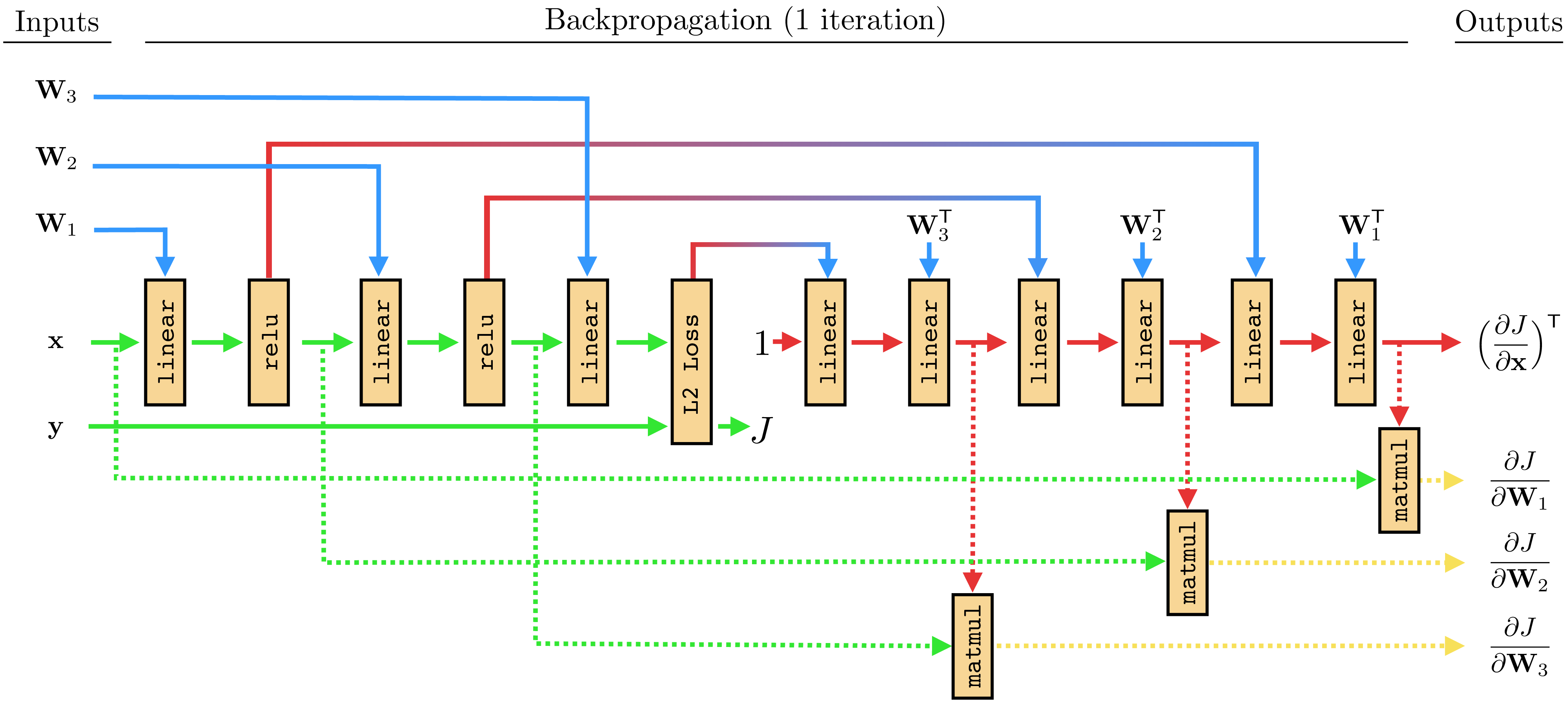
This diagram visualizes everything we've discussed.

• Forward Pass (left-to-right): The input x and labels y are leaf nodes on the left. The parameters W1, W2, W3 are also leaf nodes. They "merge" at various linear (affine transformation) and relu (activation) nodes. Finally, all paths converge at the L2 Loss node, which computes the final scalar loss value J.
• Backward Pass (right-to-left): This is a preview of our next lesson. The process starts from the loss J and propagates gradients backward through the graph. The goal is to calculate the derivatives of J with respect to the learnable parameters (∂J/∂W1, ∂J/∂W2, ∂J/∂W3), which are needed for the gradient descent update.

The structure of the graph is not always a simple chain. More complex architectures involve nodes that branch (sending their output to multiple subsequent nodes) and merge (taking inputs from multiple previous nodes). The branch operation is fundamental to how gradients are distributed, and it is how we handle concepts like parameter sharing.

Conclusion

In this lesson, we have established a powerful and general way to represent neural networks. By deconstructing the complex, nested function of a network into a computational graph, we have created a structured, modular, and scalable representation.

Key Takeaways:

• A computational graph represents a mathematical function as a directed acyclic graph (DAG) of elementary operations (nodes) and data flow (edges).
• All components of a neural network—inputs, parameters, activations, and the loss—can be laid out in such a graph.
• The forward pass involves traversing the graph from the input leaves to the final loss node, computing the value of each node along the way.
• This graphical representation is not just a visualization tool; it provides the exact structure needed to systematically apply the chain rule to every parameter in the network. Each node only needs to know how to compute its local output and its local derivative.

We now have the complete blueprint for the forward pass. The next logical step is to traverse this blueprint in reverse to compute our gradients.

In the next lesson, we will do exactly that. We will derive the backpropagation algorithm by systematically applying the chain rule backward through the computational graph, starting from the final loss and efficiently calculating the gradient for every single parameter.