Building Neural Networks: Affine Transformations & Activations

Recommended resources

The freely available resources this lesson will direct you to.

In our previous lesson, we established why multi-layer networks are fundamental to modern AI. By dissecting the XOR problem, we saw that single-layer models are confined to linear decision boundaries, while multi-layer perceptrons (MLPs) overcome this by learning to transform the input data into new, more useful representations. This is the core principle of representation learning.

Today, we will transition from this conceptual understanding to a precise mathematical description. Our goal is to formulate a feedforward neural network as a composition of functions. You will see how the entire network's computation, from input to output, can be expressed elegantly using the language of linear algebra. Each layer will be defined as an affine transformation followed by a non-linear activation, and the full network as a chain of these layer-wise operations. This formalization is the bedrock upon which we will build our understanding of network training in subsequent lessons.

The Anatomy of a Network Layer

Let's begin by formalizing the computation within a single layer. As you know from your work with linear and logistic regression, a basic unit computes a weighted sum of its inputs, adds a bias, and passes the result through an activation function. A neural network layer simply consists of many such units operating in parallel.

Your strong background in linear algebra is a significant asset here, as it allows us to express these parallel computations far more efficiently than writing out sums for each individual neuron.

Step 1: The Affine Transformation

Consider a single layer of a network. It receives an input vector $x$ from the previous layer (or from the raw data) and produces an output vector $h$ that is passed to the next layer. Let's say the input vector has dimension $n$ ( $x \in R^{n}$ ) and our current layer has $m$ neurons.

Each of the $m$ neurons computes its own weighted sum of the $n$ inputs. This can be represented by a weight matrix $W$ of size $m \times n$ , where the entry $W_{ij}$ is the weight connecting the $j$ -th input to the $i$ -th neuron in the current layer. Additionally, each of the $m$ neurons has its own bias term, which we can collect into a bias vector $b \in R^{m}$ .

The entire set of weighted sums for the layer can then be calculated in one go with a single matrix-vector multiplication and a vector addition:

z = Wx + b

Here, $z \in R^{m}$ is a vector containing the "pre-activation" values (also called logits) for each neuron in the layer. This operation, $z = Wx + b$ , is known as an affine transformation. It is a linear transformation ( $Wx$ ) followed by a translation ( $+ b$ ).

The following video provides a clear walkthrough of how we move from the neuron-by-neuron summation to this compact matrix formulation.

A Gentle Introduction To Math Behind Neural Networks and Deep Learning (nested composite function)

This video from the Dr. Data Science channel demonstrates the vectorization of a layer's computations.

Please watch the segment from this timestamp. It shows how the weighted sums for multiple neurons are elegantly captured by defining a weight matrix \mathbf{W} and a bias vector \mathbf{b}, resulting in the compact affine transformation \mathbf{W}\mathbf{x} + \mathbf{b}.

Step 2: The Nonlinear Activation

If we were to only stack affine transformations, our network would be of limited use. A composition of affine functions is itself an affine function. For example, $f_{2} (f_{1} (x)) = W_{2} (W_{1} x + b_{1}) + b_{2} = (W_{2} W_{1}) x + (W_{2} b_{1} + b_{2})$ . This is just a new affine transformation with a combined weight matrix $W^{'} = W_{2} W_{1}$ and bias vector $b^{'} = W_{2} b_{1} + b_{2}$ . Such a network, no matter how many layers deep, could be collapsed into a single layer and would still only be capable of learning linear decision boundaries.

This is why the nonlinear activation function $ϕ$ is essential. After calculating the pre-activations $z$ , we apply $ϕ$ to each element of the vector independently (element-wise). The final output, or activation, of the layer $h$ is:

h = ϕ (z) = ϕ (Wx + b)

Feed-Forward Neural Networks (DL 07)

This video by Professor Bryce explains the critical role of non-linearities in multi-layer networks.

Please watch the segment from this point. It clearly states the theorem from linear algebra that a composition of linear functions is just another linear function, motivating the need for non-linear activations to gain expressive power from multiple layers.

Composing Layers into a Network

Now we have the full mathematical description of a single layer: $f (x) = ϕ (Wx + b)$ . A deep neural network is simply a composition of these functions. The output of one layer becomes the input to the next.

Let's formalize the notation for a network with $L$ layers.

The input data is the "activation" of layer 0: $h^{(0)} = x$ .
For each layer $l$ from 1 to $L$ , we have a weight matrix $W^{(l)}$ , a bias vector $b^{(l)}$ , and an activation function $ϕ^{(l)}$ .
The computation proceeds sequentially: $h^{(l)} = ϕ^{(l)} (W^{(l)} h^{(l - 1)} + b^{(l)})$

The final output of the network is the activation of the last layer, $y^= h^{(L)}$ .

Let's write this out for a network with two hidden layers ( $L = 3$ , including the output layer):

First Hidden Layer: $h^{(1)} = ϕ^{(1)} (W^{(1)} x + b^{(1)})$
Second Hidden Layer: $h^{(2)} = ϕ^{(2)} (W^{(2)} h^{(1)} + b^{(2)})$
Output Layer: $y^= h^{(3)} = ϕ^{(3)} (W^{(3)} h^{(2)} + b^{(3)})$

Substituting the equations into each other reveals the nested, composite nature of the function the network represents:

y^= ϕ^{(3)} (W^{(3)} (ϕ^{(2)} (W^{(2)} (ϕ^{(1)} (W^{(1)} x + b^{(1)})) + b^{(2)})) + b^{(3)})

This entire expression represents the forward pass of the neural network.

The following reading formalizes these vectorized equations, and the diagram below it provides a concrete visualization.

[PDF] Lecture 5: Multilayer Perceptrons - GitHub Pages

This PDF provides a concise and formal mathematical definition of the MLP computations.

Please read the section that begins just after the hand-designed XOR example. Start at the mathematical derivation. Focus on how the initial, indexed summations (Equation 1) are cleanly replaced by the more compact vectorized form (Equation 2).

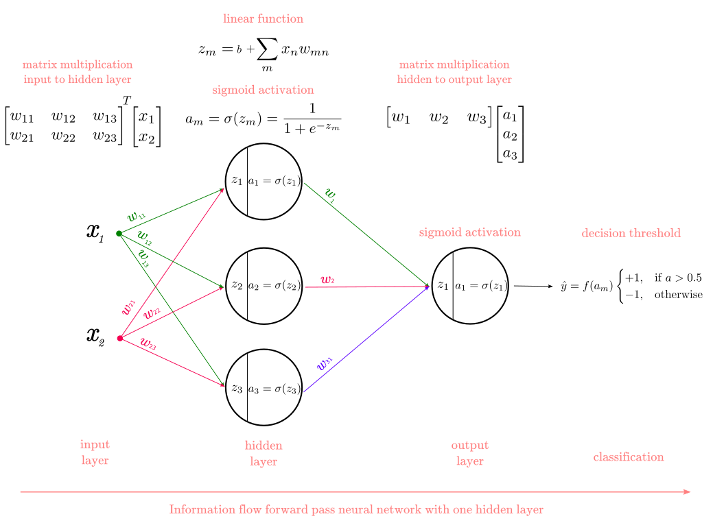
This diagram illustrates the concepts we've just discussed for a network with one hidden layer. The input vector $\mathbf{x} = [x_1, x_2]^T$ is first transformed by matrix multiplication with the weights $\mathbf{W}$ and addition of a bias $\mathbf{b}$ (the first affine step). The result is passed through a sigmoid activation to produce the hidden activations $\mathbf{a} = [a_1, a_2, a_3]^T$. This process is repeated for the output layer.

This sequence of transformations is precisely what enables the "space warping" we discussed in the last lesson. Each layer takes the representation from the previous layer and maps it into a new space, with the goal of making the final classification task easier.

This image visualizes the effect of a layer's transformation. The composition of affine transformations and non-linearities can take a dataset that is not linearly separable in its original input space (left) and map it to a new feature space where it becomes linearly separable (right).

Conclusion

In this lesson, we have moved beyond the conceptual and established the precise mathematical language for describing a feedforward neural network. This formalism is crucial for everything that follows.

Key Takeaways:

A feedforward neural network computes its output via a sequence of layers in a directed, acyclic manner.
Each layer's computation can be broken down into two steps: an affine transformation ( $z = Wx + b$ ) and an element-wise nonlinear activation ( $h = ϕ (z)$ ).
The use of nonlinear activation functions is essential; a network composed solely of affine transformations is equivalent to a single linear model.
The entire network represents a complex composite function, formed by nesting the functions of its successive layers.
The learnable parameters of the network are the collection of all weight matrices $W^{(l)}$ and bias vectors $b^{(l)}$ across all layers.

We now have a complete mathematical description of the network's forward pass. The natural next question is: how do we find the optimal values for all these parameters? This is a problem of optimization. To use an algorithm like gradient descent, we need to compute the gradient of a loss function with respect to every parameter in the network. In our next lesson, we will see how to represent our nested function as a computational graph, which provides the structural framework for efficiently calculating these gradients using the chain rule in a process known as backpropagation.