Recommended resources
The freely available resources this lesson will direct you to.
- Neural Networks From Scratch - Lec 15 - GeLU Activation Functionwww.youtube.com
- Lecture 6 | Training Neural Networks Iwww.youtube.com
- [PDF] Mathematical Analysis and Performance Evaluation of the GELU ...pdfs.semanticscholar.org
- Navigating Neural Networks: Exploring State-of-the-Art Activation Functions – OMSCS 7641: Machine Learningsites.gatech.edu
Welcome back. In our previous lessons, we've defined a feedforward neural network as a composition of affine transformations and nonlinear activation functions: . We also saw how to represent this entire computation as a graph, which sets the stage for the backpropagation algorithm.
Today, we will focus on that critical component: the nonlinear activation function, . Its choice is not arbitrary; it profoundly influences a network's ability to learn and the dynamics of the training process. We will dissect four of the most important activation functions in the history and practice of deep learning: Sigmoid, Tanh, ReLU, and GELU. For each, we will analyze its mathematical definition, its graphical shape, and, most importantly, the behavior of its gradient—a property that has driven the evolution from one function to the next.
Your strong foundation in calculus will be invaluable here, as understanding the derivatives of these functions is the key to grasping concepts like vanishing gradients and their impact on training deep architectures.
The Classic Saturating Functions: Sigmoid and Tanh
Historically, the first widely used activation functions were the Sigmoid and Hyperbolic Tangent (Tanh). They were popular partly because their bounded, "S"-shaped curves were required by early versions of the Universal Approximation Theorem, which we will discuss in our next lesson.
Let's look at their familiar shapes and formulas.

While these functions are smooth and differentiable, they share a critical flaw that hindered the development of deep neural networks. The following video explains their properties and, crucially, their drawbacks.
Lecture 6 | Training Neural Networks I
This segment from a Stanford lecture on training neural networks provides an excellent breakdown of the problems with Sigmoid and Tanh.
Please watch the following two segments: Sigmoid: Pay close attention to the two main problems discussed: Saturated gradients: Notice how the function becomes flat for large positive or negative inputs. The derivative in these regions is close to zero, which "kills" the gradient flow during backpropagation. Non-zero-centered output: The explanation of how this leads to inefficient, "zigzagging" gradient updates for the weights in the subsequent layer is particularly insightful. Tanh: Observe how Tanh solves the zero-centered output problem but still suffers from gradient saturation.
To recap the key issues:
-
Sigmoid ():
- Pros: Squashes outputs to a (0, 1) range, which is interpretable as a probability and useful in the final layer of a binary classifier. It has a direct connection to the logistic regression model you're familiar with.
- Cons:
- Vanishing Gradients: Its derivative, , has a maximum value of 0.25 at and rapidly approaches zero elsewhere. In a deep network, these small gradients are multiplied together many times during backpropagation, causing the overall gradient to "vanish" and preventing weights in early layers from being updated effectively.
- Not Zero-Centered: Outputs are always positive. As the video explained, this forces all weight gradients in the next layer to have the same sign, leading to inefficient updates.
-
Tanh ():
- Pros: Its output range of (-1, 1) is zero-centered, which resolves the inefficient update problem seen in Sigmoid. For this reason, Tanh is almost always preferred over Sigmoid for hidden layers.
- Cons: It still saturates for large , and its derivative, , also goes to zero in these regions, leading to the same vanishing gradient problem.
A Breakthrough: The Rectified Linear Unit (ReLU)
The vanishing gradient problem was a major barrier to training deep networks. The solution turned out to be surprisingly simple: the Rectified Linear Unit, or ReLU.
ReLU() = max(0, )
This function was a pivotal innovation that made training much deeper networks feasible.
Lecture 6 | Training Neural Networks I
The same Stanford lecture continues with a thorough analysis of the ReLU activation function.
Watch the segment on ReLU. The video covers its significant advantages and its primary drawback. Focus on: Advantages: How it avoids saturation in the positive region, its computational efficiency, and its faster convergence in practice. The "Dying ReLU" Problem: Understand how a neuron can become "stuck" in the negative region, where its gradient is always zero, effectively dying and ceasing to learn. The visualization of the "data cloud" is helpful for building intuition.
The success of ReLU led to several variants designed to address the "dying ReLU" problem. Here is a brief overview.
This article provides a concise written summary of ReLU and two of its important variants.
Please read the following three short sections: ReLU: This section recaps the key properties, including how ReLU induces sparsity in activations. Leaky and Parametric ReLU: These introduce a small, non-zero slope for negative inputs to prevent neurons from dying. PReLU even makes this slope a learnable parameter. ELU: This is another variant that pushes the mean of the activations closer to zero and saturates to a negative value, which can make the network more robust to noise.
In summary, ReLU and its family offered a powerful solution to the vanishing gradient problem, enabling the deep learning revolution. ReLU remains a very common and effective default choice today.
The Modern Standard for Transformers: GELU
While ReLU is powerful, modern architectures like the Transformer (which powers models like GPT and BERT) have converged on a smoother, more complex activation function: the Gaussian Error Linear Unit (GELU). Its design is motivated by combining the properties of ReLU with the stochastic regularization of dropout.
Neural Networks From Scratch - Lec 15 - GeLU Activation Function
This video from ML for Nerds offers a fantastic intuition for how GELU is derived.
Watch the first two parts of the video to understand the motivation and mathematical formulation of GELU: Intuition: Explains how GELU merges the ideas of ReLU (gating by sign) and dropout (stochastic gating). Mathematical Definition: Walks through the derivation. The core idea is that GELU is the expected value of an identity mapping x gated by a stochastic mask m \sim \text{Bernoulli}(\Phi(x)), where \Phi(x) is the cumulative distribution function (CDF) of the standard normal distribution. This leads to the definition: \text{GELU}(x) = x \cdot \Phi(x).
The exact formula for GELU involves the Gaussian error function (erf), which is computationally expensive. In practice, a very accurate and fast approximation is used. For a more rigorous look at its derivation and properties, we will turn to the original paper that proposed it.
[PDF] Mathematical Analysis and Performance Evaluation of the GELU ...
This paper provides the rigorous mathematical treatment you appreciate. It will give you a deep understanding of GELU's design.
Please read the following sections: Section 2.2, "GELU Activation Function" (full section): This details the motivation as a smooth alternative to ReLU and provides the full derivation, starting from the Gaussian CDF, \Phi(x), and ending with the common tanh-based approximation: \text{GELU}(x) \approx 0.5x(1 + \tanh(\sqrt{2/\pi}(x + 0.044715x^3))). Section 3.1.1, "Derivative of the GELU Function" (this subsection): This section provides the full derivation of GELU's derivative using the product and chain rules. Pay close attention to the analysis of its implications. Unlike ReLU, the gradient is non-zero and even slightly negative for some negative inputs. The authors argue this can help the model escape local minima during early training.
The key insight is that GELU acts as a smooth, probabilistic version of ReLU.
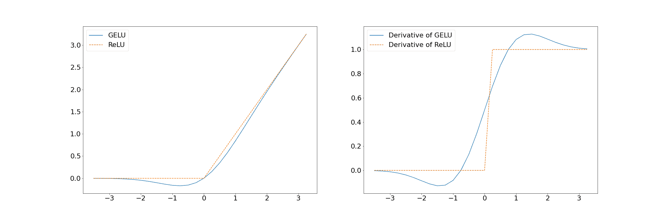
As the plots show, for positive inputs, GELU closely tracks the identity function, similar to ReLU. For negative inputs, it gently curves towards zero but doesn't have the hard zero "kink" of ReLU. Its derivative is smooth and continuous, peaking above 1 and having a small negative lobe, which contrasts sharply with ReLU's simple step-function derivative. These properties contribute to more stable and effective training in large-scale models.
Conclusion
We have journeyed from the historical sigmoid function to the modern GELU, seeing how the evolution of activation functions has been driven by the need to solve critical problems in training dynamics, particularly the vanishing gradient problem.
Key Takeaways:
- Sigmoid and Tanh are "saturating" functions whose gradients vanish for large inputs, making it difficult to train deep networks. Tanh is an improvement over Sigmoid because its output is zero-centered.
- ReLU provided a major breakthrough with its non-saturating positive part and computational efficiency. However, it can suffer from the "dying ReLU" problem where neurons become permanently inactive.
- GELU is a smooth, differentiable approximation to ReLU, motivated by stochastic regularization. Its non-monotonic shape and smooth gradient are thought to contribute to its superior performance in state-of-the-art Transformer models.
Here is a summary table for comparison:
| Function | Formula | Range | Zero-Centered? | Vanishing Gradients? | Key Pro/Con |
|---|---|---|---|---|---|
| Sigmoid | (0, 1) | No | Yes (severe) | Con: Kills gradients and has non-zero-centered output. | |
| Tanh | (-1, 1) | Yes | Yes (saturates) | Pro: Zero-centered. Con: Still kills gradients. | |
| ReLU | [0, ) | No | No (for ) | Pro: Efficient, no saturation on positive side. Con: Can "die". | |
| GELU | (-0.17, ) | Mostly | No | Pro: Smooth, performs well in Transformers. Con: Complex. |
In our next lesson, we will step back from the practical properties of these functions to address a more fundamental question: why does introducing any of these nonlinearities give neural networks their power? We will explore the Universal Approximation Theorem, which provides the theoretical foundation for the expressive capacity of neural networks.