MOS Amplifier Biasing

Recommended resources

The freely available resources this lesson will direct you to.

Introduction

In our recent lessons, we have developed a solid foundation in the analysis of MOSFET circuits. You've learned how to determine a transistor's operating region, calculate its drain current, and find the DC operating point (Q-point) for various configurations, including those with active loads. We have been answering the question: "Given this circuit, what are its DC voltages and currents?"

Today, we transition from analysis to design. This lesson focuses on the inverse problem: "Given a desired DC operating point, how do we design a circuit to achieve it?" Your learning objective is to master the design of bias circuits for discrete MOS amplifiers to set a specific Q-point. This is a fundamental skill for any analog circuit designer, moving from simply understanding circuits to creating them. We will focus on the most common and robust topology for discrete amplifiers: the four-resistor voltage divider biasing network.

The Goal of Biasing Design

Before we jump into calculations, let's clarify our objective. The goal of biasing is to establish a stable DC operating point—defined by the quiescent drain current $I_{D Q}$ and drain-source voltage $V_{D S Q}$ —that places the transistor firmly in the saturation region. This prepares the MOSFET to amplify a small AC input signal without distortion.

A common design strategy is to place the Q-point to allow for the maximum possible symmetrical swing in the output voltage. A good rule of thumb is to set the DC drain voltage, $V_{D Q}$ , roughly halfway between the supply voltage ( $V_{D D}$ ) and the source voltage ( $V_{S}$ ). This gives the AC signal equal "room" to swing up and down before hitting the supply rails or driving the transistor into the triode region.

The video below provides an excellent overview of different biasing methods and reinforces why the voltage divider configuration is a practical and stable choice.

MOSFET Biasing : Enhancement Type MOSFET Biasing Explained

This video, "MOSFET Biasing : Enhancement Type MOSFET Biasing Explained" from ALL ABOUT ELECTRONICS, explains the need for biasing and compares different techniques.

First, watch the introductory segment on the need for biasing to refresh your understanding of why we must operate in the saturation region for amplification. Then, jump to the section explaining the voltage divider bias. Pay close attention to the circuit analysis using KVL and the intuitive explanation of how the source resistor, R_S, provides stability.

The Voltage Divider Biasing Circuit

The circuit discussed in the video, shown below, is our focus for today's design task. It uses four resistors ( $R_{1}, R_{2}, R_{D}, R_{S}$ ) and a single power supply $V_{D D}$ to establish the Q-point.

The standard four-resistor voltage divider biasing circuit for an n-channel MOSFET. Our goal is to calculate the values of $R_1, R_2, R_D$, and $R_S$.

The design process is a systematic application of Ohm's Law and the MOSFET I-V characteristics, working backward from the desired operating point.

A Step-by-Step Design Procedure

Let's outline the logical sequence for calculating the four resistor values. Assume we are given the target Q-point ( $I_{D Q}$ , $V_{D S Q}$ ) and the transistor's parameters ( $V_{T}$ and the conduction parameter $k_{n}$ ).

Determine $R_{D}$ and $R_{S}$ : These resistors are found by applying Ohm's law to the output loop (the drain-source side of the circuit). Knowing the target currents and voltages makes this straightforward.
Determine the required $V_{GS}$ : Using the saturation current equation, we calculate the gate-source voltage $V_{GS}$ needed to produce the target drain current $I_{D Q}$ .
Determine the required Gate Voltage $V_{G}$ : With $V_{GS}$ and the desired source voltage $V_{S}$ known, we use KVL to find the necessary DC voltage at the gate terminal.
Determine $R_{1}$ and $R_{2}$ : Finally, we design the resistive voltage divider to produce the target gate voltage $V_{G}$ from the main supply $V_{D D}$ .

The following reading provides a complete, worked example that follows these exact steps. It's an excellent resource for seeing the entire process from start to finish.

MOSFET Amplifier Circuit using an Enhancement MOSFET

This article from Electronics Tutorials provides a very clear, step-by-step guide to designing a common-source amplifier's bias network.

Please read the section titled "MOSFET Amplifier Worked Example". It starts with a problem statement and methodically calculates all the component values, R_D, R_S, R_1, and R_2, to meet a specific biasing condition. Follow each step carefully and see how it maps to our design procedure.

Design Walkthrough: A Practical Example

Now, let's apply this procedure ourselves to a typical design problem. Your experience with circuit analysis will be very helpful here, as we are essentially using the same equations, just solving for different unknowns.

Consider the following design challenge:

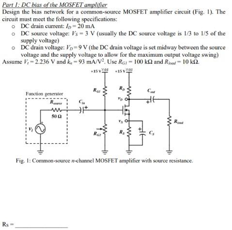
Design problem for a common-source amplifier. We need to find the values for the biasing resistors.

Given:

Supply Voltage, $V_{D D} = + 15 V$
Transistor parameters: $V_{T} = 2.236 V$ , $k_{n} = 93 mA/V^{2}$

Design Specifications (Target Q-point):

DC Drain Current, $I_{D} = 20 mA$
DC Source Voltage, $V_{S} = 3 V$
DC Drain Voltage, $V_{D} = 9 V$

Let's follow our four-step process.

Step 1: Calculate Drain and Source Resistors ( $R_{D}, R_{S}$ )

We apply Ohm's law to the drain and source circuits. We know the current through each resistor is $I_{D} = 20 mA$ , and we know the voltage drop across them.

Source Resistor $R_{S}$ : The voltage across $R_{S}$ is $V_{S} - 0 V = 3 V$ .
$R_{S} = \frac{V _{S}}{I _{D}} = \frac{3 V}{20 mA} = 150 Ω$
Drain Resistor $R_{D}$ : The voltage across $R_{D}$ is $V_{D D} - V_{D} = 15 V - 9 V = 6 V$ .
$R_{D} = \frac{V _{D D} - V _{D}}{I _{D}} = \frac{6 V}{20 mA} = 300 Ω$

First two resistors found. Let's also verify that the transistor is biased in saturation at this Q-point.
The drain-source voltage is $V_{D S} = V_{D} - V_{S} = 9 V - 3 V = 6 V$ . We will compare this to $V_{GS} - V_{T}$ in the next step.

Step 2: Calculate Required Gate-Source Voltage ( $V_{GS}$ )

We need to find the $V_{GS}$ that will produce our target drain current of 20 mA. We use the saturation current equation:
$I_{D} = \frac{1}{2} k_{n} (V_{GS} - V_{T})^{2}$
Solving for $V_{GS}$ :
$V_{GS} = \frac{2 I _{D}}{k _{n}} + V_{T}$
$V_{GS} = \frac{2 \times ( 20 \times 1 0 ^{- 3} )}{93 \times 1 0 ^{- 3}} + 2.236 V$
$V_{GS} = 0.4301 + 2.236 V = 0.656 V + 2.236 V = 2.892 V$
So, we need a $V_{GS}$ of approximately 2.89 V.

Now we check the saturation condition: Is $V_{D S} \geq V_{GS} - V_{T}$ ?
Our $V_{D S}$ is 6V. The overdrive voltage $V_{GS} - V_{T}$ is 0.656 V.
Since $6 V > 0.656 V$ , the transistor is indeed well into the saturation region, and our design is valid.

Step 3: Calculate Required Gate Voltage ( $V_{G}$ )

The gate-source voltage is defined by the potentials at the gate and source terminals: $V_{GS} = V_{G} - V_{S}$ . We can rearrange this to find the required gate voltage.
$V_{G} = V_{GS} + V_{S} = 2.892 V + 3 V = 5.892 V$

Step 4: Calculate Gate Bias Resistors ( $R_{G 1}, R_{G 2}$ )

Our final task is to choose $R_{G 1}$ and $R_{G 2}$ to create a voltage divider that provides $V_{G} = 5.892 V$ from the 15V supply. The problem statement gives us a helpful constraint: Use R_G1 = 100 kΩ. This simplifies our task, as we only need to solve for $R_{G 2}$ .

The voltage divider equation is:
$V_{G} = V_{D D} \frac{R _{G 2}}{R _{G 1} + R _{G 2}}$
Plugging in the known values:
$5.892 = 15 \frac{R _{G 2}}{100 k Ω + R _{G 2}}$
Now we solve for $R_{G 2}$ :
$5.892 \times (100 k Ω + R_{G 2}) = 15 R_{G 2}$
$589.2 k Ω + 5.892 R_{G 2} = 15 R_{G 2}$
$589.2 k Ω = (15 - 5.892) R_{G 2}$
$589.2 k Ω = 9.108 R_{G 2}$
$R_{G 2} = \frac{589.2 k Ω}{9.108} \approx 64.69 k Ω$
In practice, you would choose the nearest standard resistor value, such as 64.9 kΩ (1% tolerance) or 68 kΩ (5% tolerance).

Our design is complete! We have found the values for all four resistors:

$R_{S} = 150 Ω$
$R_{D} = 300 Ω$
$R_{G 1} = 100 k Ω$
$R_{G 2} \approx 64.7 k Ω$

A Note on Bias Stability

It's worth reinforcing why this four-resistor circuit is so widely used. Its stability comes from the source resistor, $R_{S}$ , which introduces a form of negative feedback.

channel MOSFET Transistor

This lab manual from the University of Kentucky provides a concise explanation of bias stability.

Find the circuit diagram in Fig. 3 and read the two bullet points directly below it. These points explain how the circuit achieves a stable DC operating point. Focus on the explanation of how the source resistor R_S provides negative feedback.

This self-correcting mechanism makes the Q-point less sensitive to variations in temperature and transistor parameters like $k_{n}$ and $V_{T}$ , which can vary significantly between devices, even of the same part number.

Conclusion

This lesson marked an important shift from circuit analysis to circuit design. By working backward from a set of performance specifications, you learned how to systematically determine the component values for a robust MOSFET biasing network.

Here are the key takeaways from our design process:

Design starts with the Q-point: The desired quiescent current ( $I_{D Q}$ ) and voltages ( $V_{D Q}, V_{S Q}$ ) are the starting point.
The process is systematic:
1. Calculate output loop resistors $R_{D}$ and $R_{S}$ using Ohm's Law.
2. Calculate the required $V_{GS}$ from the MOSFET saturation equation.
3. Determine the target gate voltage $V_{G}$ using KVL.
4. Design the input voltage divider ( $R_{1}, R_{2}$ ) to produce $V_{G}$ .
The four-resistor topology is stable: The inclusion of a source resistor $R_{S}$ provides negative feedback, making the Q-point resilient to parameter variations.

You have now completed the first major module on MOSFET DC analysis and biasing. With the ability to both analyze and design the DC operating point of an amplifier, you are fully prepared for the next step. In our next module, we will investigate how these properly biased transistors behave when an AC signal is applied. We will begin by introducing a "small-signal model" for the MOSFET, starting with a non-ideal effect called channel-length modulation, which gives the transistor its characteristic output resistance.